In my last post I showed you two ways of creating a new wireframe from a set of XYZ points. Both methods were slightly more involved than what is really necessary but illustrated some useful tools that may come in handy at other times.  In this post we will cover some different, simpler methods for achieving the same aim. Jun will cover the process in Leapfrog Mining; I will cover the process in Geo. For something different and by way of introduction I will finish by describing the process using Micromine’s new Implicit Modelling process as a comparison to Leapfrog products.

Leapfrog Mining
In Leapfrog Mining, there is a simple way to assign polarity to a set of points so that 'inside' and 'outside' of an object can be defined easily.  Once this is done, the points can be correctly interpolated and the surface reconstructed from the points.

For example, when a topography point set is imported into Leapfrog Mining, the software does not know how to join the points, so it searches through the points and assigns a positive and negative sides to the set of points by adding many "off-surface" value points. The mechanics and logic of this process is described in an earlier post on topographic modelling. This process is automated for modelling topography, but what is commonly not known by Leapfrog Mining users is that a topography point set can also be interpolated by simply adding a single point with polarity using the point drawing tool in 3D drawing mode.  There is no need to section the data in 2D, but you simply add a point with polarity by viewing and digitising in the tangential view of a local topography surface continuity.  You then merge this point with the polarity data with the original topography points and you can interpolate the topography surface.   This is an elegant method as it takes only one point to define the polarity, and that is all that is needed to model other sheet-like surfaces such as faults.

Similarly, this process can be used to model more complex 3D set of points, and this is the method that I would use in Leapfrog Mining to model the set of points under consideration (Figure 1).


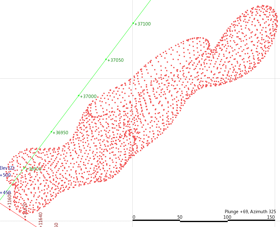Figure 1. A point cloud imported into Leapfrog - in this case it is extracted points from a mesh discussed in Part 1 of this post.


To do this, you simply have to identify an area where the local surface does not curve around too much, and then add a point with polarity using the 3D polyline tool (Figure 2, 3). 


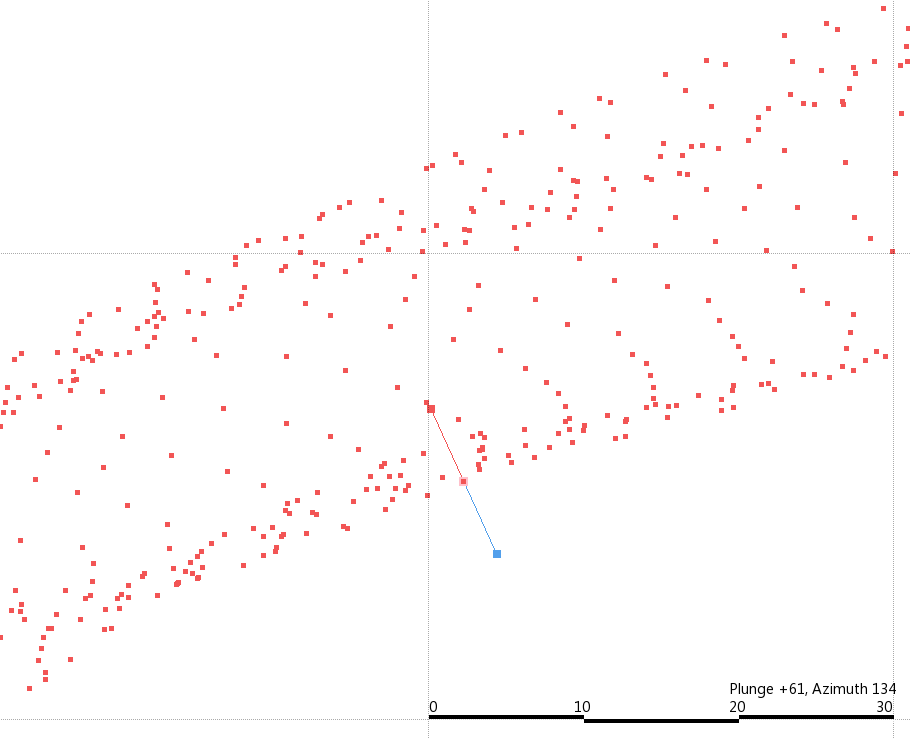Figure 2. A point with polarity handles drawn on a point in 3D view (not sectioned). Note that the view is tangential to the surface being modelled (i.e looking along within the surface) so that the polarity handles are approximately orthogonal to the surface defined by the points.



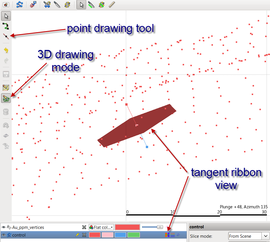Figure 3. The point with polarity handles in an oblique view.  The tangent position should be turned on and assessed to see if it is positioned correctly.

When you draw this point be sure to be viewing in the tangential orientation of the imagined surface defined by the points (i.e looking along within the surface).  This way the point normals when they are drawn out will be in the correct orientation.

There is no need to 2D section the model at all, but you work entirely in 3D mode.  If you turn on the polyline tool, then the point drawing tool will by default stick onto the nearest point and as long as you are viewing along the local tangent of the surface you are trying to model, then all you need to do is to draw the point normals out to orthogonal to the surface being constructed to define the positive side being in the inside of the point set (as a rule, I define inside of objects as positive).  Once you draw in one point, turn on the first ribbon icon to check the tangent surface of the point (Figure 3).  If this tangent it cutting across the surface defined by the points at a high angle, then redo the point so that the ribbon is a tangent surface.  Repeat the drawing process in another part of the object (perhaps to define the surface on the other side) and you end up with two control points (Figure 4), or alternatively you may want to use polylines instead of points, but whatever you do, you must be in tangential view of the surface being modelled during digitisation (There is a simple geological reason why this 3D drawing tool was designed this way, but that topic will be for another blog post).


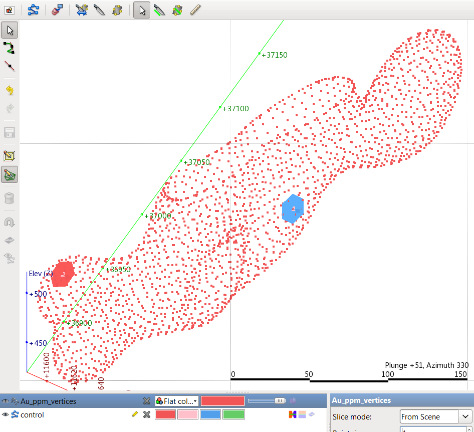Figure 4. After digitising two control points that help to define the 'inside' and 'outside' of the point data.  The polarity is displayed as coloured disks with red facing inwards and blue facing outwards.

Once you digitise the control points, you save the point set and the familiar off-surface value points will be generated along with the interpolant and the surface.  The only feature that we need to use is the off-surface points located straight under the polyline icon in the project pane.



Right click on this and select 'merge objects', and you will then be able to merge this dataset with the original set of points (Figure 5).  This merged dataset is interpolated resulting in the modelled object from the data (Figure 6).


Figure 5. Merge Objects dialogue box showing both the original data and the off surface points that were created from the two control points shown in Figure 4.


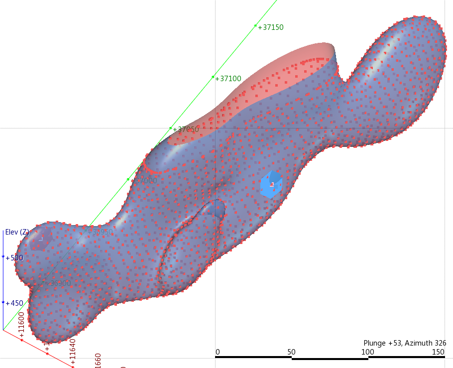Figure 6. Modelled surface in Leapfrog Mining using two points as control.

Leapfrog Geo
Unlike in Leapfrog Mining we cannot digitise points in Leapfrog Geo, to achieve the same result we either utilise structural data or we can digitise a couple of lines to achieve a similar result. Last time we generated the wireframe we used multiple structural data points, we can actually achieve the same result using just two points, especially when the shape is defined by a large amount of data. The procedure is exactly the same as outlined in the previous post but we simply create 2 points rather than many, one on either side of the shape, and ensure the positive side of the structural disks face inwards (Figure 7).


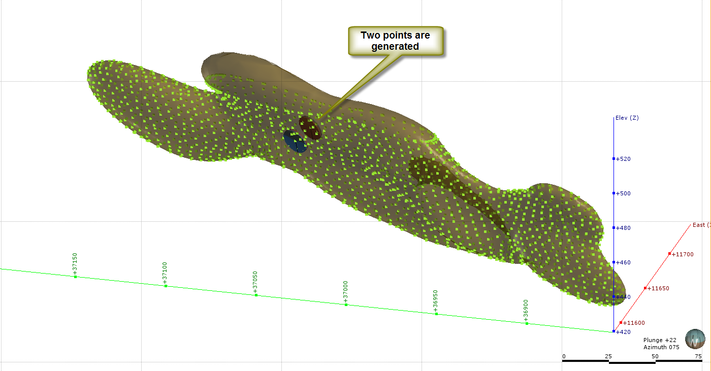Figure 7.  We can use just two structural points  to create the normals we need to build the wireframe.

The other method is to use the polyline. There is an option to Edit the mesh using a polyline once the mesh has been built. When you do this keep in mind that the normal of the polylines will align with the section and not with the direction of view as it does in Mining, therefore you must ensure your section aligns with the view before you use this option. Having said that, don’t bother trying this method as it will not work anyway. Editing the mesh using this option will not affect the alignment of the normals, it just adds more points into the mix. In order to define the normals to drive the shape we need to digitise the line separately. To do this we follow the following procedure;

1. We cut a section through the shape, this should be normal to the dip of the shape we are trying to model. Then right click on the Polyline folder and select New Polyline. This asks for a file name and activates the drawing tool.

2. Digitse two lines on either side of the shape you wish to model (Figure 8). These lines need only be short and consist of two points.

 

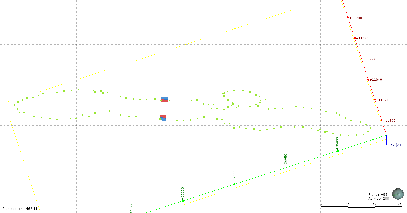
Figure 8. Digitise two lines on either side of the shape, they need only be short. Note that these polylines can only be drawn in 2D section so they are not physically snapped to any of the points.

3. In order to define the normals we must extract these points as Structural points, we do this by right clicking on the polyline and selecting Estimate Structural Data...

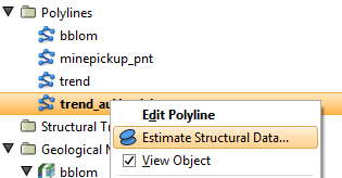
This will extract the points as structural points, with the normals taken from the normals on the polylines. From this point it is simply a case of creating the mesh and adding the structural data as per Part 1 (Figure 9). So why would you bother digitising a line if you have to convert it to structural points anyway? Good question, there may be reasons as to why you need the line but it would be easier to generate two structural points if this will achieve the result. 


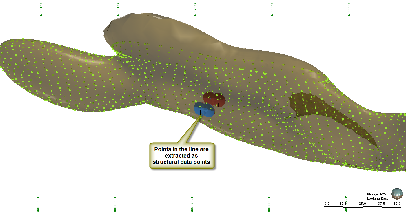Figure 9. Extracting the lines as structural points allows you to utilise the normals in defining the shape.

Micromine IM
As many of you will be aware Micromine has recently brought out an implicit modelling module (IM), this was covered by Jun in his post Six reasons why Micromine’s new implicit modelling software could triumph over Leapfrog. I am currently working on a Leapfrog – Micromine comparison with I will post shortly but thought this would be an interesting problem to use as a way of introducing IM in Micromine. One could say the process is actually easier in Micromine as there is no reason to digitise anything to derive the shape.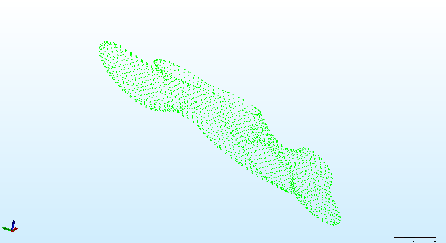


Figure 10. The same dataset in Micromine.

The implicit Modelling module sits under the Modelling Menu item. To generate the shape we use the Point Cloud option. This option is used to model both surfaces and 3D shapes – or “Point Clouds”!


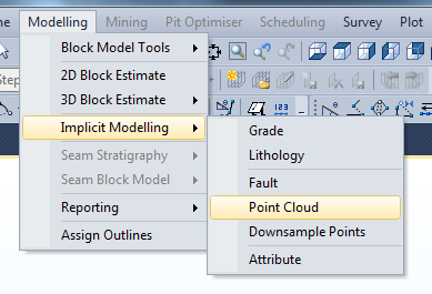
This brings up the Point Cloud modelling form (Figure 11). The first Input/Output tab is where we define the input points and the output wireframe with colours and mesh sizes. The Build Options tab is where we define the modelling parameters. The parameters of note are the Number of Neighbours and the Max points per neighbourhood. The number of neighbours is what MM uses determine the shape – is it an open surface or a closed shape, in particular it is used to define the normal or direction perpendicular to the surface which determines up from down, inside from out. The Max points per neighbour is what is used by MM’s modelling method to determine the surface shape. These settings can be a bit of trial and error to settle onto a final setting but on a simple shape like this it does not take long to rebuild the shape.



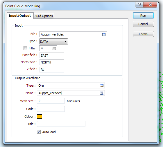
Figure 11. The Micromine Implicit Modelling Point Cloud option opens a window with two tabs used to define the shape, these are the settings I have used to model the shell.

Upon clicking the Run button MM goes and processes the shape (Figure 12). I had to re-run the process a couple of times adjusting the main parameters to obtain a satisfactory result. One thing you will note is that MM’s implicit modelling process is a memory hog and the machine will bog down while it processes. Not an issue on a small dataset but it will stop you from multi-tasking on larger datasets while the computer thinks.
 

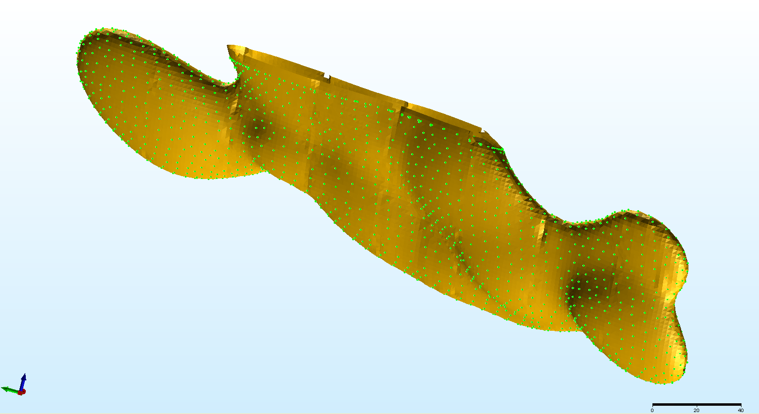
Figure 12. Final product using the MM implicit modelling process.

As you can see the result is quite satisfactory when compared to the output from Leapfrog (Figure 12), a couple of artifacts that could probably be fixed by fiddling with the parameters but overall a good result. The lack of a requirement to digitise anything is perhaps off-set by the need to run a couple of times to settle on correct parameters, practice with the process allows you to eyeball the required parameters and reduces the need to re-run.

There you have it, several methods in three programs for achieving the same result. Increasing complexity can make the process more difficult and sometimes the result you are after may not be achievable, however when it comes down to needing to re-digitise the lot – if a little bit of IM magic works it saves a whole lot of pain.

Of particular note is the usability and results from Micromines new Implicit modelling module which is only early in its development.

Certainly the Micromine's IM module will be a force to be reckoned with in the future.

----

Keep an eye out in the near future for a more complete review of Micromine IM product by Ron Reid!