Occasionally you have a requirement to create a new volume wireframe from a set of xyz points. They may represent a survey pick up of a stope or perhaps you have extracted the points from a mesh and wish to recreate the wireframe. Recently I was asked to review a deposit that had a corrupted domain wireframe – but the point file associated with it was OK. This got me thinking of the different ways I could re-create the DTM using Leapfrog after importing the point file. In this, the first part of a 2 part piece I will discuss two different methods of generating a mesh from a set of points. In Part 2 we will present additional methods for achieving the same result. We hope to show you that there are many ways of achieving the same outcome, each with a different approach, and each with its unique set of steps (and hurdles) that you may recognise as being useful in other areas of your modelling. Like many Leapfrog Mining users I have been struggling with the new layout and workflows of Leapfrog Geo and thought I might also show you some methods we can use to recreate a mesh using Geo. In the process I will introduce the generation of a Leapfrog block model and flagging the model with our domain. I will leave the grade estimation and reporting for a future post but will cover the creation of reporting domain here.

The scenario involves taking an exported set points that a colleague has sent, asking if we can calculate an average grade inside this shell using some drill hole information (Figure 1).




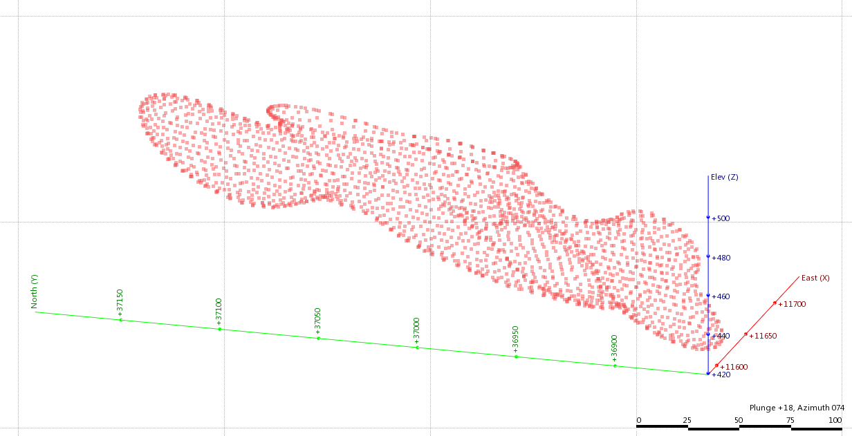Figure 1. A point cloud imported into Leapfrog - in this case it is extracted points from a mesh.

Normally the first step is to import the drill hole information which I touched upon in a previous post (Basic grade interpolation in Leapfrog). We will not require the drilling data for this post so I will not cover it here. The next step for us is to import the csv of the point data. I will cover the process in Leapfrog Mining first, then repeat the process using Geo.

Leapfrog Mining

Step one involves importing the data as a new boundary file by right clicking on Boundaries and selecting Import…. Navigate to your file, select it and import. This will simply import the XYZ file and leave you with a point file under your Boundaries folder. You can validate this by dragging it into the viewer (Figure 1). At this point you may try to either generate a Surface Interpolant or Triangulation. You will find you will fail to obtain any useful wireframe (Figure 2). To enable us to generate a realistic shape we must first tell Leapfrog what is inside and what is outside (or what is positive and what is negative).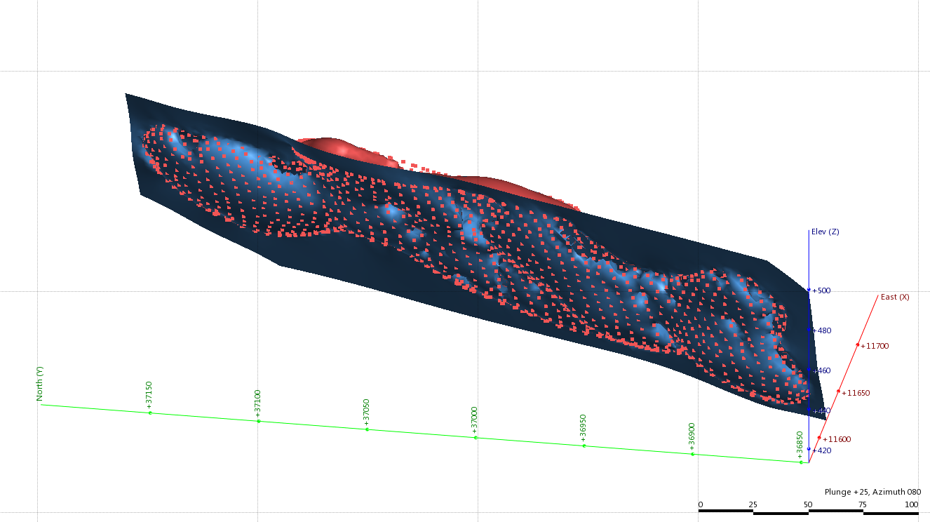





Figure 2. You can not recreate a wireframe by simply generating an interpolant (top) or a triangulation (bottom).


To do this we must generate Surface Values. If we were to simply generate these however we will get a strange result (Figure 3). This is because Leapfrog assumes you are looking down and you are generating surface values on a flat surface. To generate a volume we first we need to tell Leapfrog what is inside the set of points and what is outside to achieve a useful outcome (Figure 3).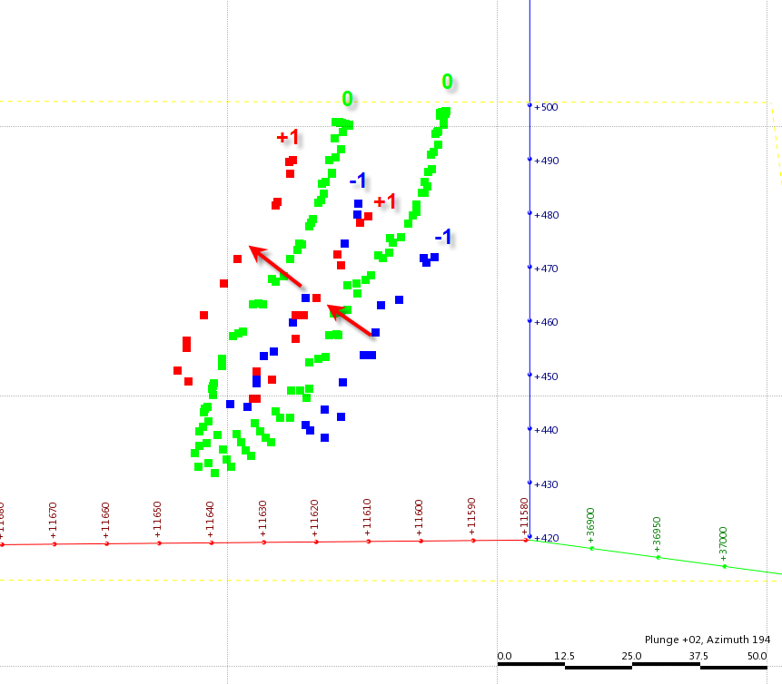





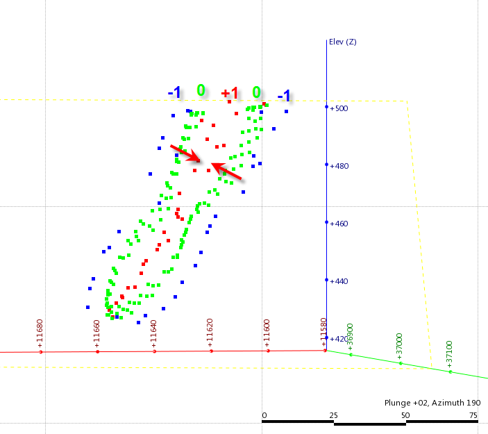
Figure 3. If you generate the surface values straight up you will get an erroneous result (top), we need a result that will show us what is inside and what is outside the wireframe (bottom).


One way to do this in Mining is to generate a distance interpolant, create a distance shell, use this to create a structural trend and then use this structural trend to map out the positive and negative values. To do this we can follow this procedure;

1. Obtain a dip, dip azimuth and pitch of the points using the plane tool (Figure 4)
2. Create a distance interpolant (right click on the point values and select Distance Interpolant…), fill the global trend using the Set from Plane button and select OK.
3. Generate a distance mesh on the shell that approximates the shape of the point cloud. I used a distance that was approximately the width of the shell, in this case 25m (Figure 5). The actual distance is not that significant however you do not want a mesh inside your domain, hence the use of the total width as a measure.
4. Once you have a shell you can create a structural trend using this buffer (right click on Structural Trends, select New Trend… (Figure 6). I have found the best results come from using the strongest along meshes option but a little trial and error will help you find what works best for you.
5. Once you have a structural trend you can generate your surface values, this time selecting your structural trend under the Use normal from trend: option. I have trailed with various degree settings and found something between 20 to 45 degrees works best, this is a trial and error setting and will be specific to the shape and complexity of your domain.
6. Once you have created the surface values, you can create the new mesh, right click on the surface values file and select interpolate values…
7. Under the grade parameters tab set the clipping to a narrow band of say -1 (or -0.5) for the lower bound and +1 (or +0.5) for the upper, this ensures the mesh more closely honours the data. Select the structural trend option under the variogram tab, this will activate the Spheroid variogram option. Set the range to around 1 third of the strike length of your shell, and the nugget to around 10-25% (have a play, the larger the number the smoother the result). Run this and assess the results, you may have to play with the mesh resolution, etc but the result should be closely match the original points. It will not be exact but will be close enough for the purposes of an evaluation (Figure 7).
   
   

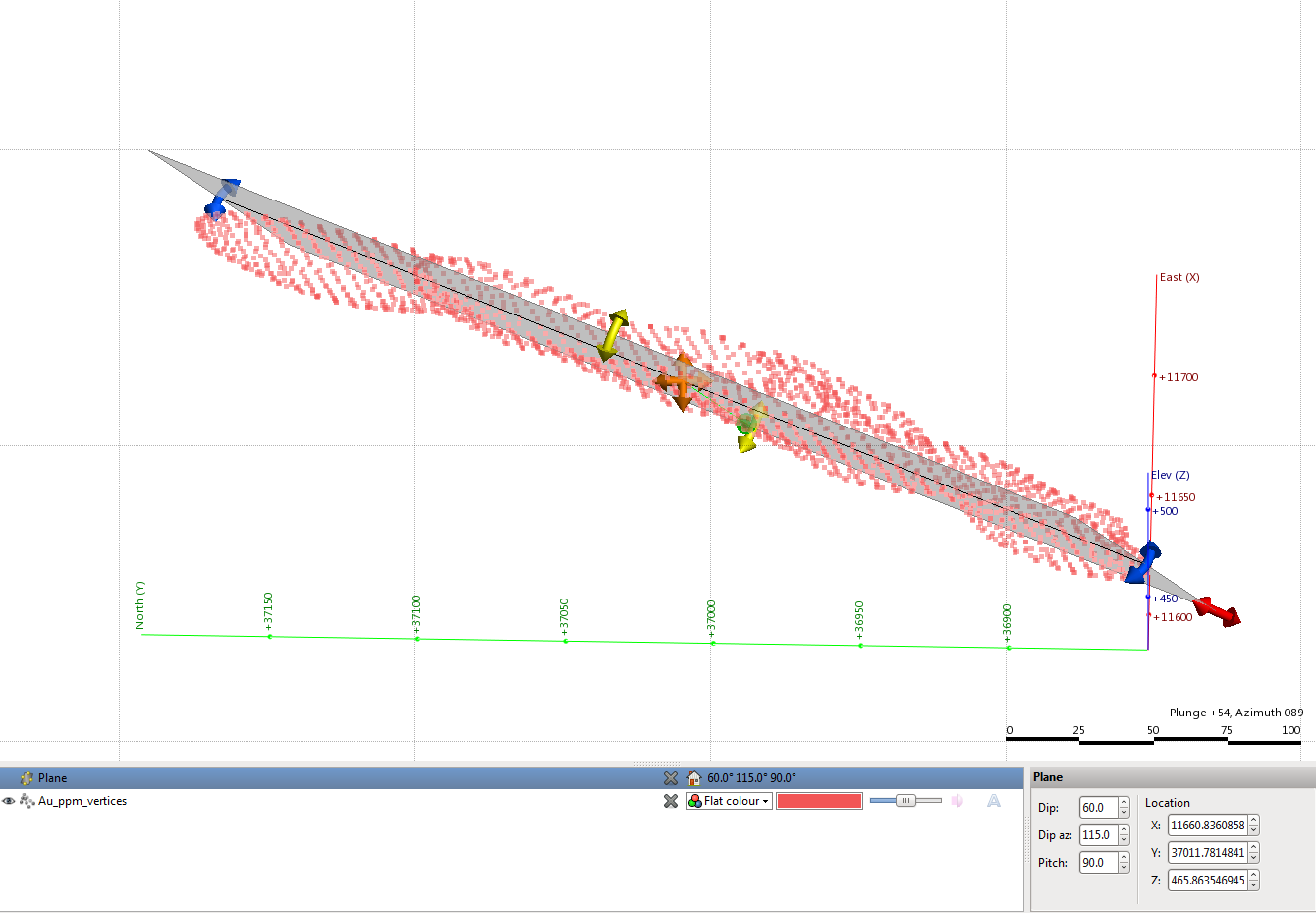Figure 4. Obtain a trend of the data using the plane tool.



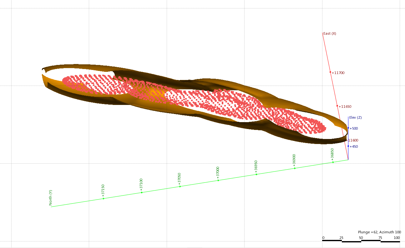Figure 5. A distance interpolant around the points at 25m.





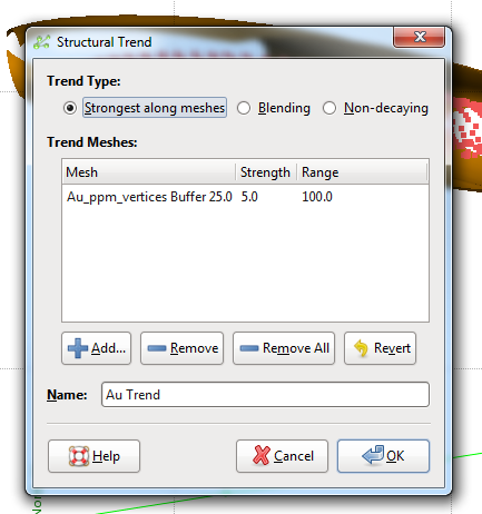
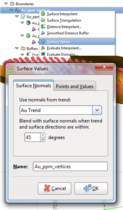Figure 6. Create a new structural trend by selecting the buffer mesh created from the distance interpolant (top). Once this has been done you can select this structural trend in surface values form (bottom).



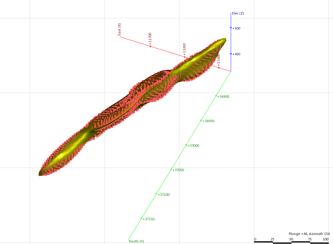Figure 7. The final domain shell should closely match the original points.


You can then use this interpolation to define a domain (Figure 8), right click on Domains and select Define Domain…, then select the interpolant for your mesh and give it a meaningful description. Once you have this you can use it to generate a subset of composite points, use it to constrain an interpolation, and evaluate a grid of points.





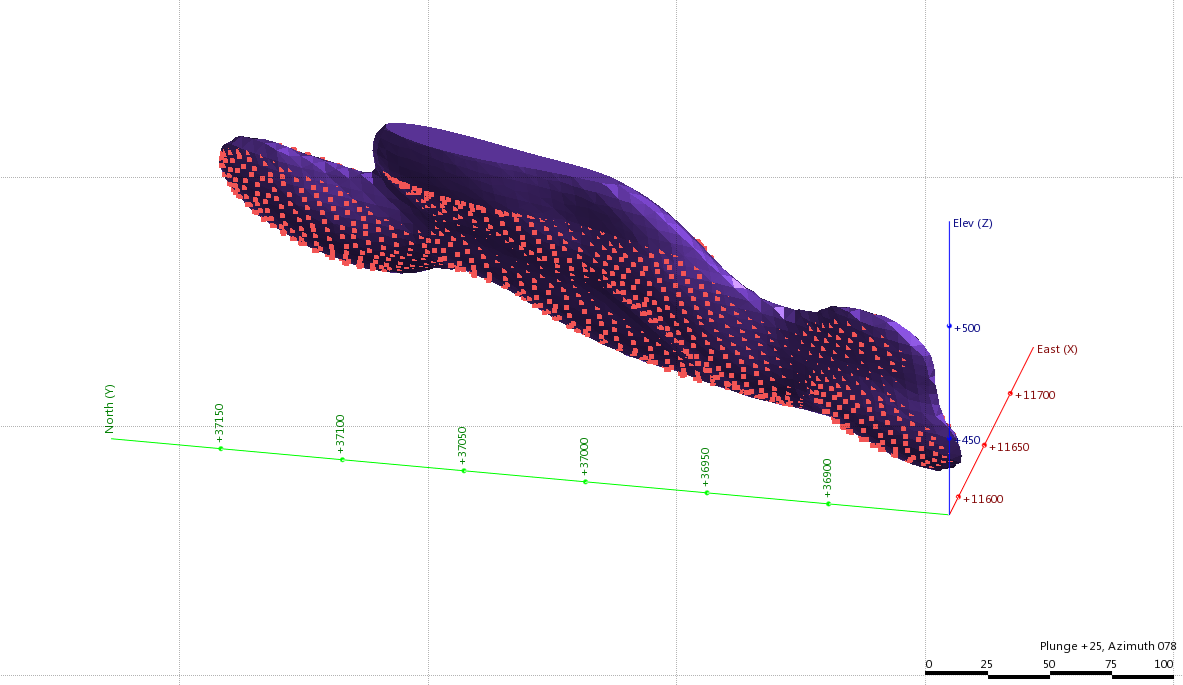Figure 8. You can use the resulting interpolant to define a domain that can be used to create a subset of assay data, and evaluate against a grid of points.


To create a Leapfrog block model you create a new Grid of points, right click on Numeric Data and select either New Grid of Points, or New Orientated Grid of Points. I always use New orientated grid of points as it gives you more flexibility in setting up the grid, whilst I generally do not rotate the model (ever mindful of the heart palpitations this causes mining engineers) I find I have more control over setting up my model simply using this option. Be aware that unlike most GMP packages where the bottom south west corner is defined by the base point (as either the centroid or cell corner), in leapfrog it is the Top southwest centroid. This is signified in Leapfrog with the orange crossed arrows. Once you have set up your grid of points you can evaluate the domain by right clicking on the grid and selecting domain evaluation, then select the domain (I always use the interpolant rather than the mesh) and you now have a flagged block model. This is a simple domain and of course multiple domains can become quite complex but the principle remains the same. If you evaluate the grid against an interpolant and then export the data you can create Grade tonnage curves and report the tonnes and grade above various cut-offs for different domains, however I will leave that for a future discussion.




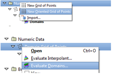
Figure 9. Figure showing the creation and evaluation of a grid of points on the top, and the resulting grid inside the domain on the bottom.

Leapfrog Geo

The process in Leapfrog Geo is a bit different but will give you the same result as Mining (as will attempting to generate a mesh without following this procedure). The first step is to import the data into the locations folder (right click on Locations and select Import Locations…). Once you have the data you can do the following;

1. Cut a section or plan and generate some structural data (right click on Structural Data and select New Structural Data). Digitise some structural points on several Slices that give you a positive (red=inside) and negative (blue=outside) side to the point data (Figure 10). You do not need many of these, just enough to roughly define the shape.
2. Create a new mesh (right click on Meshes, select New Mesh, then From Points…), the result will be ugly but this is the first step.
3. Once the mesh has been built, right click on the new Mesh and select Add, then Structural Data, then select your new structural data file. The mesh will rebuild and will look much more like your point cloud (Figure 11). 
4. You can tidy up the mesh by right clicking on the Mesh, selecting Open and the adjusting the Trend, Value transform and variogram (Interpolant) as you would in Mining.
5. A simpler process at the start than in Mining, defining the domain however involves a few more steps. First you create a New Geological Model and call it Domain, set the base Lithology column: to <None>, and set a resolution commensurate with your mesh. Adjust your domain boundaries to fit with your working area. Make sure that if your shell is open (as it is here) you must ensure the top boundary of the geology model intersects the open part of the mesh (or that the open part of the mesh intersects the topography), else you will get an error.
6. Once your model has been built you right click on Boundary and select New Lateral Extent and then From Surface…, then select your domain mesh. This will generate an ‘unknown’ volume that defines the domain (Figure 12). You can then select this domain when generating an interpolant to constrain the interpolation to within the domain or to flag a grid of points, I will cover the grade interpolation in a future post, but discuss the creation of a grid of points below. The domain will remain as ‘unknown’ as you can not currently rename the unknown rocktype, hopefully Leapfrog will address this feature in the future.
   
   

Figure 10. Generate some structural data measurements that will be used to generate the mesh.


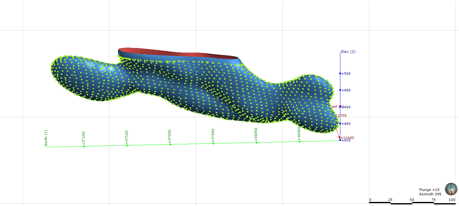Figure 11. The final mesh should resemble your point cloud.


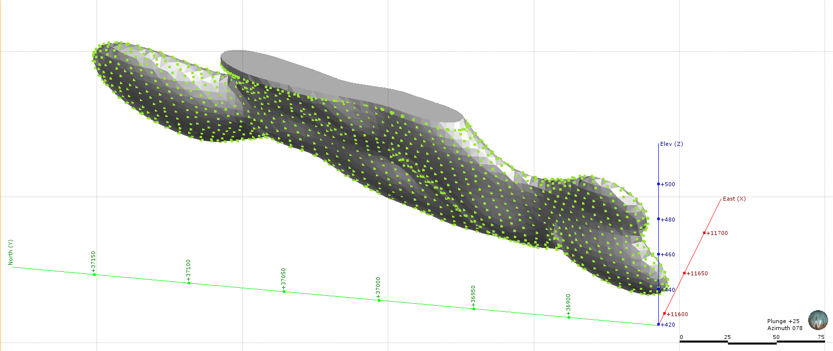Figure 12. A new geology model called Domain with one unknown rock type - this is the domain.


You can create a grid of points in LF Geo 1.3 or later by right clicking on the Locations folder and selecting New Grid of Points (Figure 13). This set up works the same as it does in Mining, allowing you good control on the extents of the model. The evaluations of domains (in the this case it says Evaluate Geological Model) and the evaluation of numerical Interpolants is much the same, although in Geo you can combine different geological models and sort by order of precedence, allowing you to evaluate several different “domains” at the same time. Useful for where faults may break up the deposit into different models as you have less fields to assess in your block model. Be aware that at this stage in Geo you cannot see what you have evaluated against your grid of points unless you have it loaded into the view, also as the default colour for ‘unknown’ is white you may not see anything when you first load your grid, changing the colour of your unknown rock type will allow you to see the grid (Figure 13).





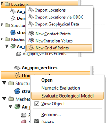
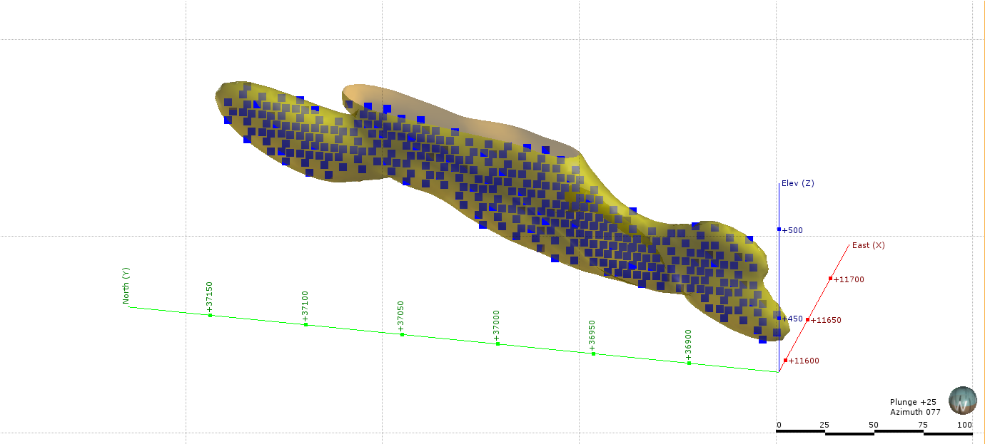Figure 13. Creating a grid of Points in Leapfrog Geo.


And there you have it, a rebuilt mesh with which to carry on your evaluation, have a play with your own data. As stated at the start of this post Jun and I will bring you Part 2 in the near future where we will cover two different methods (one each for Mining and Geo) of achieving the same result. Some may wonder if you can use the Mining method discussed above in Geo, and visa versa – Give it a go.


Cheers
Ron