In my post on topographic contours I recommended using post-processed LIDAR (or other high-quality survey point data) and interpolating this data in 3D to obtain the most accurate topographic surface for 3D modelling. I don’t see the sense in using the derivatives (contours or 2D grids) for 3D modelling purposes when a company has access to the original point data. Although I didn’t specifically point this out, the use of derived data (i.e. contours or 2D grids) for 3D modelling is common in the exploration and mining industry.

However, for the sake of brevity I didn’t explain the difference between 2D and 3D interpolation, thus prompting the following comment from Brian Grant (from Vancouver via LinkedIn).

“Seems like a pointless argument based on data resolution not 2D vs 3D. But I do agree that higher resolution surface data (e.g. LIDAR) is a wonderful supplement for geological interpretation and especially since many GIS systems can deal with LIDAR surfaces.”

Since most geologists are unfamiliar with true 3D interpolation, I will elaborate further in this and future posts, as it is quite involved. The flavour of 3D interpolation that’s used in Leapfrog Mining has many applications and I will cover these in detail in future posts. For today, I will illustrate the stark difference between 2D and 3D interpolation.

Please note that the results in this post show modelling results from Leapfrog Mining version 2.4.5.17.  The release version of Leapfrog Geo is built in a way that it cannot show the details discussed here (particularly, the 'off-surface points' which I discuss below).  The details in Leapfrog Geo are either hidden so that it cannot be accessed by the user, or it is simply deleted.  This is apparently to minimise confusion, but instead of educating the user, ARANZ Geo has taken the easy path of making Leapfrog Geo into a black box.

A good place to start is to describe the 2D interpolation methods and modelling; again, I’ll use the LIDAR topographic data introduced in my topographic contour post.

Traditional methods of topographic interpolation are 2D

There are two traditional methods to produce a topography surface from survey points such as LIDAR, and both are 2D methods. Please note: The term ‘2.5D’, commonly seen in software marketing material, is nothing more than 2D interpolation; i.e. elevation expressed as a function of X,Y position.

One simple method to model topography from LIDAR is a direct triangulation of the point data (Figure 1), which involves connecting neighbouring points with straight lines to form a triangulation surface; the software repeats this for all points until all points are connected (Figures 2, 3). As long as there are no multiple elevation values at a given X,Y coordinate, this method is very quick because the process doesn’t require any interpolation. However, your computer may suffer in performance when displaying these surfaces if large LIDAR point datasets (i.e. several million points) are triangulated. Even if triangulation of the points is possible, you may not be able to render and work with such a dense dataset on your desktop computer.


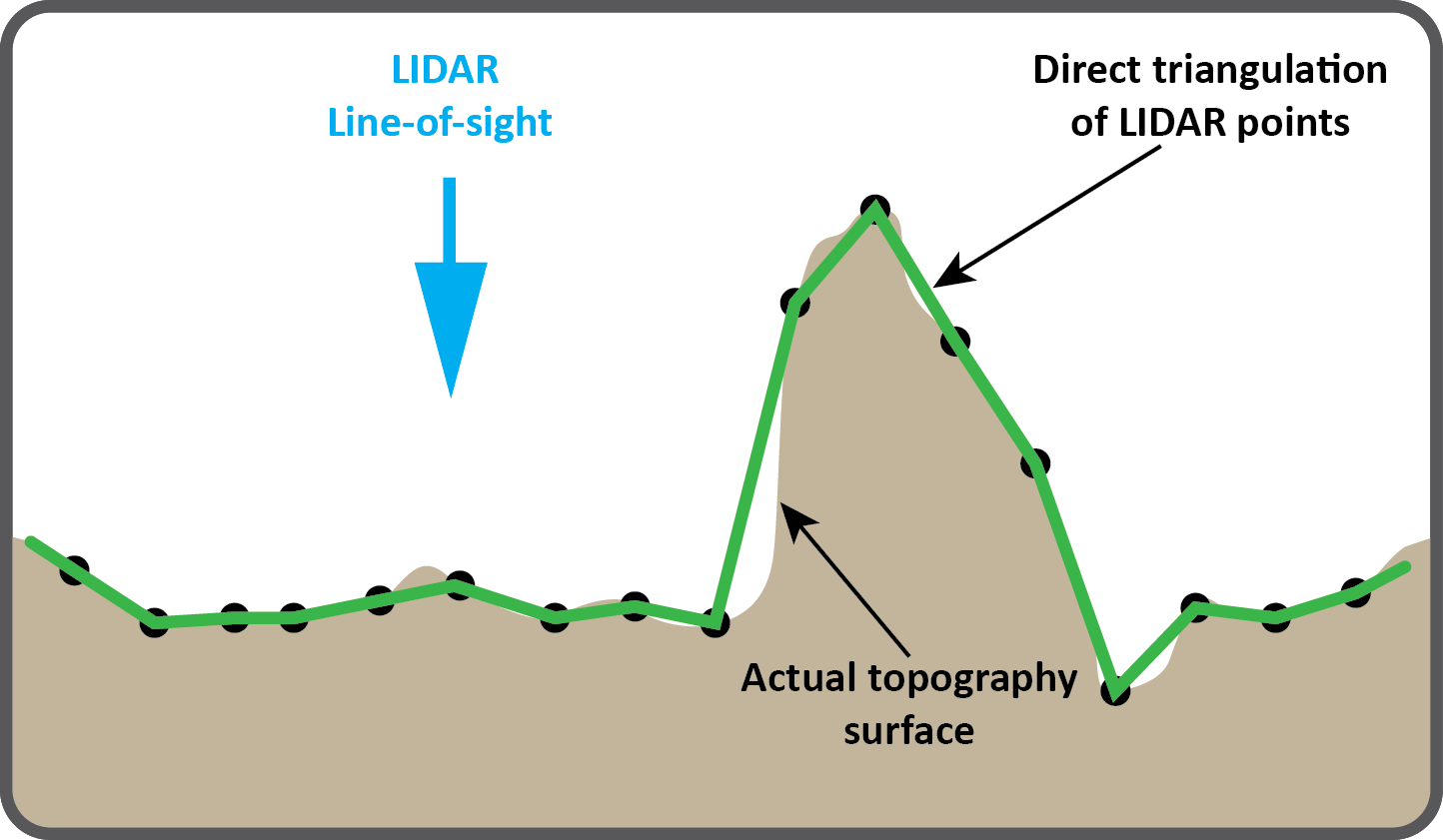Figure 1.  Cross-sectional view of a hilly terrain with schematic representation of the triangulation of LIDAR points shown as black dots. This 2D method won’t work if there are multiple points along the ‘line-of-sight’ axis (in this case vertical).

When a direct triangulation is made, you will notice that the triangles that are joined up along steep faces are stretched out (Figure 3), as the Z-axis is the default line-of-sight for triangulation of LIDAR data. Most generalised mining software products will let you to specify this line-of-sight, or projection line. This simple 2D methodology makes triangulation of rangefinder point data, with an inclined line-of-sight, possible. Regardless of the orientation of the line-of-sight, no points can hide behind other points along this projection line, otherwise this 2D triangulation method won’t work.
 

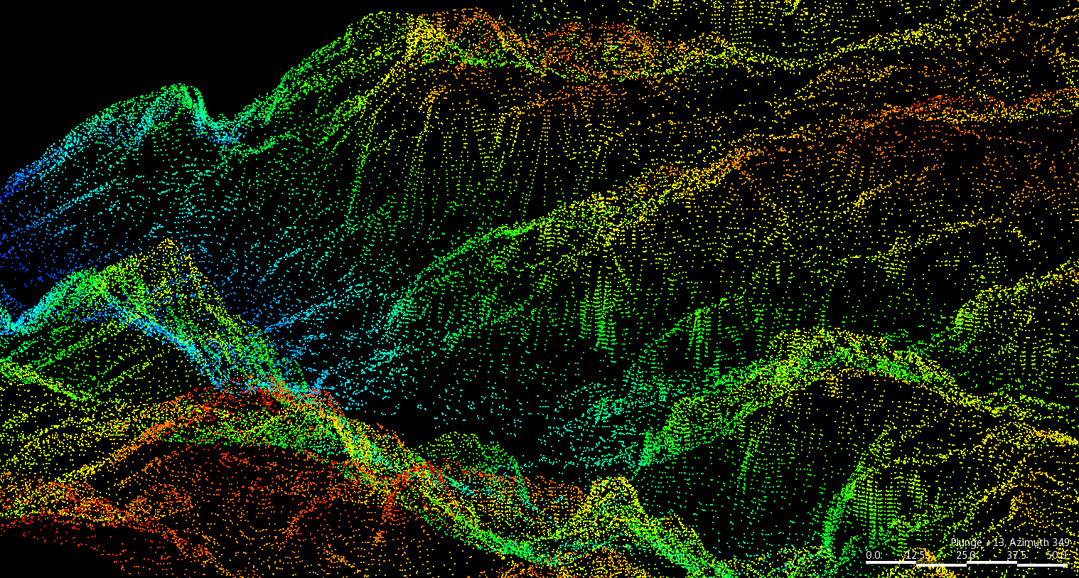Figure 2.  Original LIDAR point data.



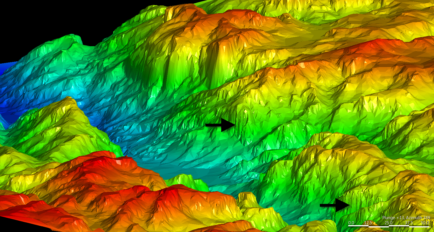Figure 3. Triangulation surface of the original LIDAR points using the vertical axis as the projection line. This is sometimes referred to as the TIN surface. Note the long triangle facets on steep slopes (arrowed).

Another drawback of the triangulation method is that it can’t reduce noise that may exist in the acquired data, so instead of a generalised surface, which may be a smooth best-fit surface that goes through the densest part of the point cloud, every survey point is reflected in the final mesh. Any noise in the data (unexpected peaks and troughs) becomes part of the topography surface.
Another method is to interpolate the points in 2D; i.e. assuming that the elevation is a function of X,Y position. Elevation values are saved in a grid of X,Y coordinates. Various interpolation methods can be used, with nearest neighbour (Figure 4 ) and inverse distance (Figure 5) methods commonly available. This method doesn’t reflect the points, but it does generate a generalised surface, although the outputs tend to be step-like, especially where there are steep hills. If accurate modelling of steep cliffs and peaks is required, then the output must be in a fine enough grid resolution to allow this detail to be imaged. With 2D interpolation, reducing the mesh resolution again creates a large file size output of the entire topography surface, but it doesn’t necessarily improve the appearance of that topography (Figure 6).


Figure 4. Nearest neighbour method of 2D interpolation. 2 m resolution grid.


Figure 5. Inverse distance method of 2D interpolation. 2 m resolution grid.
 

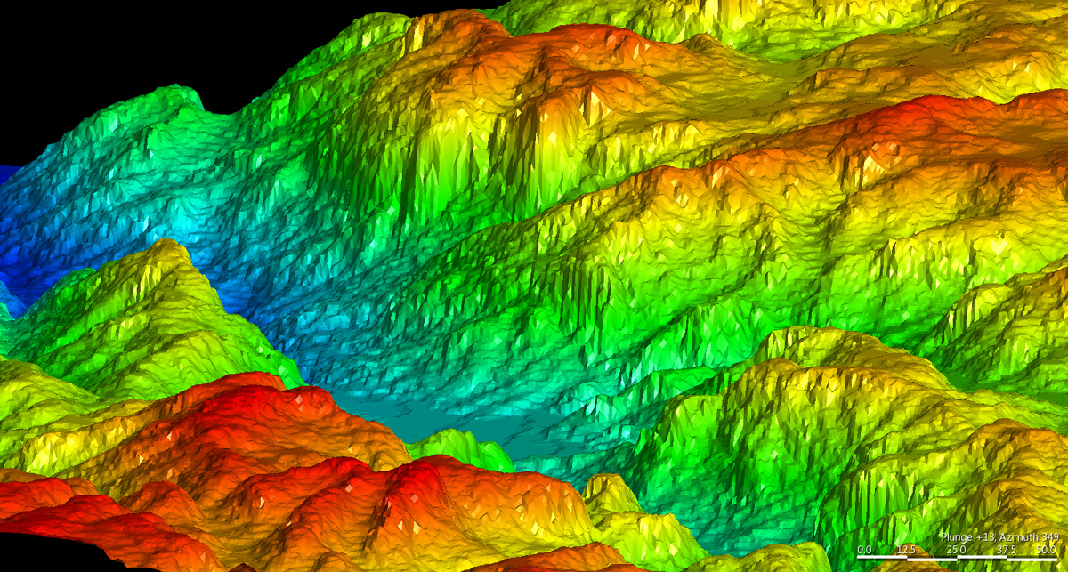
Figure 6. Inverse distance method of 2D interpolation. 1 m resolution grid. Elongated triangular facets on cliff faces will never disappear, even at high resolutions.

The main drawback with 2D interpolation is that it may not be possible for other high-quality point datasets to take advantage of the simple 2D functional relationship. These would include photogrammetry data points, such as those produced with Sirovision; underground cavity monitoring systems; or survey point-clouds generated from multiple rangefinders.

For example, consider point-cloud data obtained from two rangefinders’ views (Figure 7). The 2D interpolation method can work on a single view rangefinder dataset as long as the Z direction is rotated parallel to the laser’s line-of-sight. With most software products, the user can specify in which direction to look to ‘join the dots’ (i.e. a projection line), so the direction of 2D triangulation doesn’t have to be vertical. This method, of course, can be implemented on a single laser scan dataset with a single view direction.
 

Figure 7. Cloud data and direct triangulation of survey points obtained from several rangefinders’ orientations. Each scan can be triangulated separately by using the line-of-sight as the projection line. Typically, the total point set can’t be combined from several scans of differing orientations as some points will repeat along a chosen projection line for triangulation.

However, if you combine several rangefinder point datasets from multiple directions you end up with a dataset that has no single view line that can be used to triangulate the data. Modelling a best-fit surface from this type of composite point-cloud data using a 2D method gets really complicated and you can’t produce a continuous surface easily. This is because surface position is a function of X,Y and Z, and, for a given X,Y coordinate (a 2D relationship only), there are multiple intercepts of the surface we’re trying to model.

The Delicate Arch example

A good example of acquiring rangefinder data from multiple views is described in this 25 February 2012 post written by an Autodesk expert about scanning, modelling, and 3D printing of the well-known Delicate Arch in Utah. The data used to model this natural sandstone arch was composite point-cloud data obtained from rangefinders positioned at multiple view directions so that the arch could be accurately sampled from all sides. The author admits that modelling a surface from the composite point-cloud data was tricky, although he does not describe the exact details of how this was achieved. He writes:

“Getting the point cloud from a laser to a surface watertight meshed model is no easy feat especially with an organic structure as faceted as the sandstone arch and currently requires a great deal of work and various software. Hopefully in the future this becomes an easy process.”

My interpretation of that statement is that ‘it would be convenient if there was a general 3D method to model objects of any shape and a method that could work on any type of point-cloud data and that we no longer had to be limited by the 2D limitation’. What this author didn’t know was that a tool for this type of modelling has been available for more than ten years. I found it in 2001 using a Google search, which then led to the development of Leapfrog software, but that’s another story for another post. At Leapfrog’s core is a rapid 3D interpolation engine; the following describes the setup of the data and how that contrasts with 2D interpolation methods.

Conversion of ‘dumb points’ to 3D points

When 2D interpolation is conducted, each X,Y point has an elevation value as a variable, which is interpolated as a function of the X,Y position.

For 3D interpolation of points in space, you must assign a variable for each X,Y,Z point, but it cannot be the elevation value, as that’s used as the Z-value of the point. Effectively, these points don’t have a variable assigned to them, so I refer to them as ‘dumb points’ as you can’t interpolate points without the values.

From the original dataset, a new set of points is created offset orthogonally to the point-cloud cluster and then assigned an orthogonal distance value from the original points (Figure 8). Points generated on one side of the surface are assigned positive distance values, and on the other side are given negative distance values. Because these additional points are effectively away from the original surface points, they are referred to as ‘off-surface’ points (Figure 9).
 

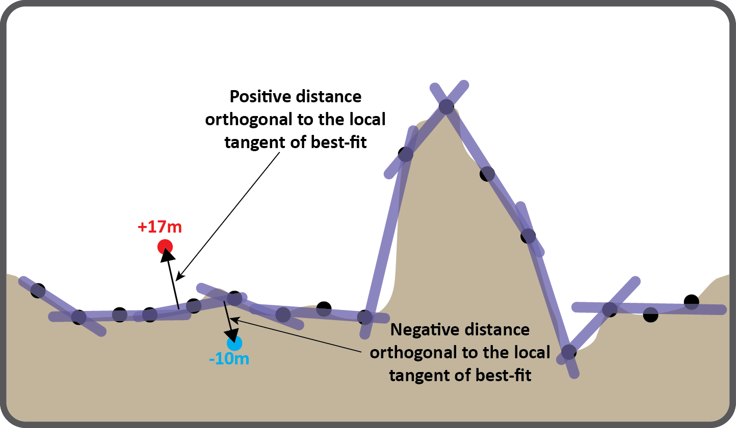
Figure 8. Best-fit tangents disks are fitted locally to points and then ‘off-surface’ points are created as shown. These off-surface points are assigned a distance value that is orthogonal to the local tangent. By default, the distance above the topography is positive and below is negative.
 

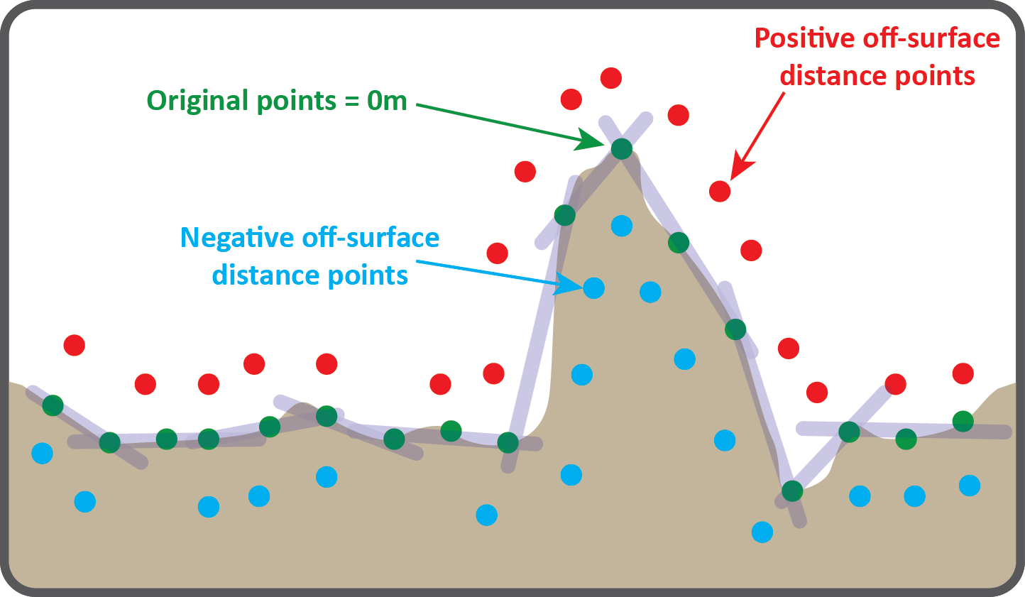
Figure 9. The original survey points are shown in green, and they are assigned a value of 0. The red and blue points are positive and negative off-surface points, respectively.

Once you’ve expressed the distance from the erosion surface as a function of X,Y,Z, when you interpolate these values you end up with a volume function with a positive region and a negative region, and the contact between these regions is the 0-value surface in the case of LIDAR, which represents the topography surface (Figures 10, 11).
 

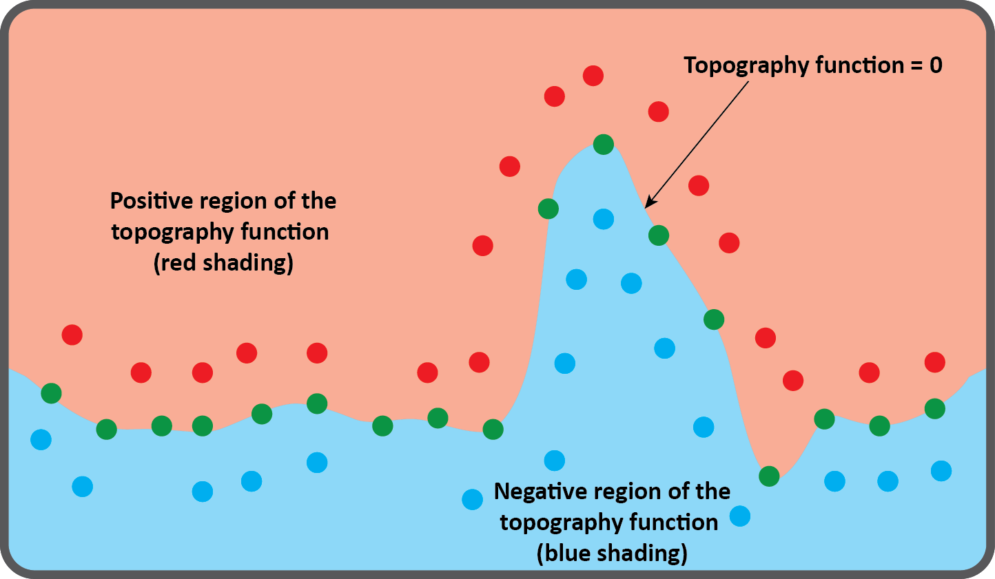
Figure 10. Once the points are interpolated, it results in a 3D function that consists of positive and negative volumetric regions. The contact between these regions is the 0-value surface and this represents the topography surface in the case of LIDAR as input data (green points).
 

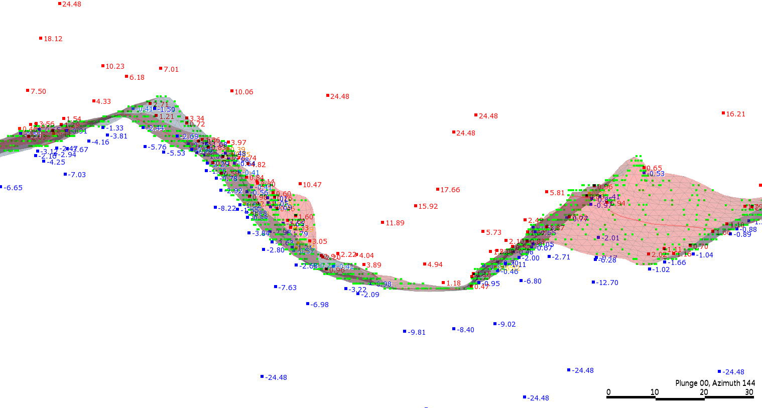
Figure 11. Sectional detail of off-surface points with positive (red) and negative (blue) distances and the interpolated topography surface of the original LIDAR data (green points).

Understanding this step is quite crucial as numerical points that allow modelling of lithology from drillhole data are prepared in a similar way. The main advantage of this method is that the topography surface position is now not just a function of X and Y, but also Z. Actually, it is the 0-value 3D contour of a continuous volume function. The 0-value isosurface is then extracted from this function; this is what you can use as the topography surface, and you can do this at any resolution (Figures 12 - 15).


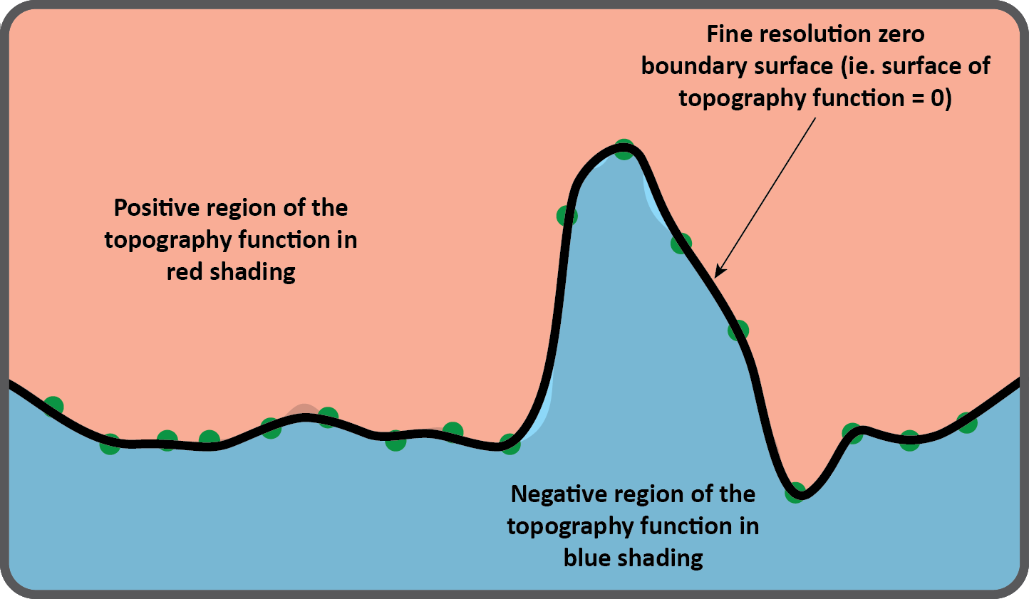Figure 12. Topography surface can be extracted from the smooth function at a high resolution.


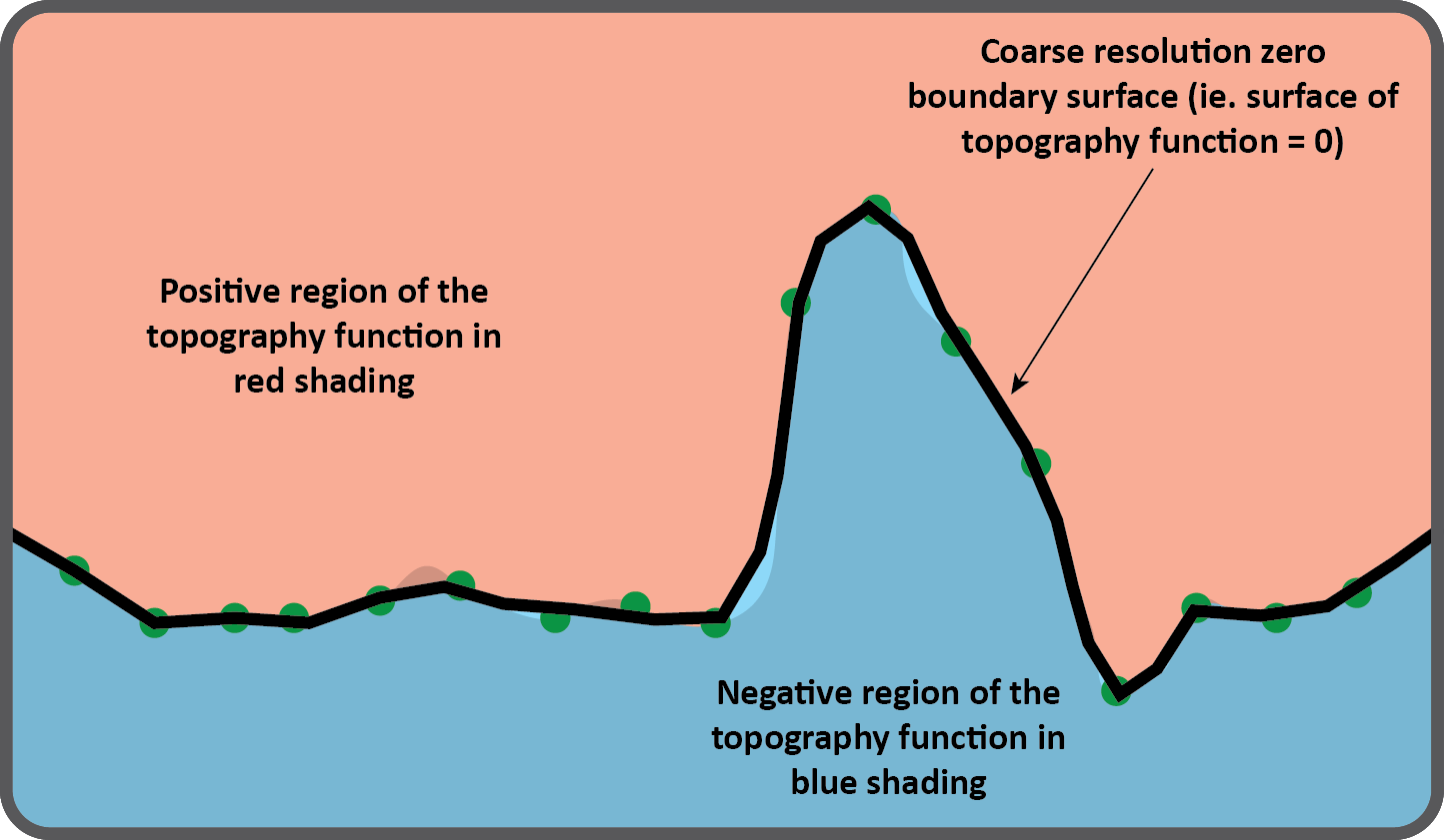
Figure 13.  Topography surface can be extracted from the smooth function at a low, or coarse resolution.

The quality of these full topography surfaces from 3D functions are very good, with high resolution detail still possible on steep cliffs (Figures 14 and 15). These details are simply not possible to achieve with the 2D method of topographic modelling, which has thin triangular slivers on steep cliffs (Figures 3 to 6).
 

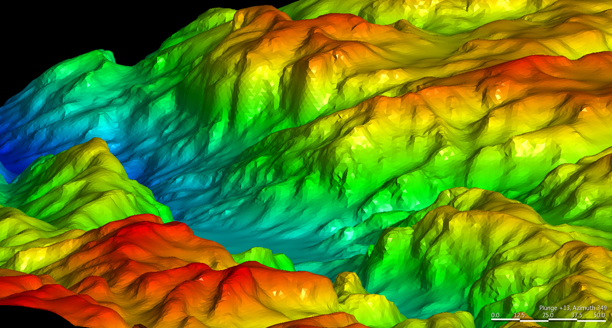
Figure 14. 2 m resolution full 3D topography surface created with Leapfrog Mining.
 

Figure 15. Multi-resolution full 3D topography surface created with Leapfrog Mining.

The imperfections seen in steep cliffs are a result of the LIDAR data being 2D data only.
This is despite the fact that LIDAR data capture is 2D, so the resolution on steep surfaces will always be limited compared to the horizontal (thus the imperfections seen in Figure 15), but this is not always the case if you’re dealing with laser point data obtained from ground level. For example, 3D interpolation would have been a natural choice to model the multiple scan rangefinder data of the Delicate Arch in Utah mentioned earlier.

Some of you may be wondering how I deal with dense data such as LIDAR. I’ll deal with this issue in a third part of this series of posts on modelling topography.

Acknowledgement: Ron Reid kindly processed the 2D grid models shown in Figures 4 to 6 using Micromine software.