This post is a follow on from my Boundary Analysis in Leapfrog blog posts and a response to a Micromine Forum question asking how to complete the boundary analysis in Micromine. Micromine is the only other general mining product (GMP) I know that can flag points with the distances normal to a mesh although I am open to being corrected if anyone knows of any others that can do the same. The workflow is simple and pretty much follows the same process for Leapfrog Geo as seen in my slide presentation but can be done entirely within Micromine.

The first step is to have your wireframe you wish to test and a composite file to flag. Remember that boundary analysis can be easily corrupted by improper data selection. Mixing of boundaries is the most common form of data "pollution" where you may be testing a lithological contact but have neglected to exclude data that may be affecting the result such as an oxide boundary or fault for instance. For this reason use Micromine's mesh Boolean options to define a volume with which to flag your data that excludes other contaminating boundaries (Figure 1).


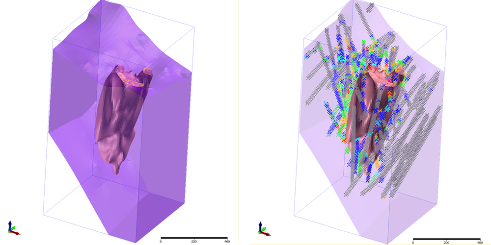Figure 1. Generate the relevant domain excluding all distracting boundaries - here on the left I have created a volume below the oxide horizon and above a thrust. On the right I have created a subset of the composites that are clipped to the purple domain which I will use to evaluate the distance from the porphyry internal to that domain.

The wireframe I have used was created using Micromine's Implicit Modelling process but it could be any implicit or explicitly modelled surface or solid. Note that in Figure 1 there is no data above or below the porphyry that might unduly influence the evaluation. With the data and wireframes in hand the actual workflow is outlined below.

At this point you can flag your composite file with distances from a wireframe using Wireframe ->  Calculations -> Distance from Wireframe  (Figure 2).  There is a lot of information that can be obtained from this form that makes it quite a useful calculation to run. The most important information to record are Distance and Position. The distance is a positive distance between the point and the wireframe surface, it is always positive whether it is from the inside or outside surface. To obtain positive and negative distances you use the position field and code +1 for inside and -1 for outside (or +1 for above and -1 for below when using a surface). For a closed (and valid) solid Outside limits is simply outside the wireframe, for a surface it represents all those samples beyond the extent of the surface - seeing as we have limited our composites to a specific volume if you are using a surface there should be no points beyond the extent of the wireframe and so you need not worry about it. The other options are nice to have and quite useful from a validation point of view - they are the name of the wireframe used (useful when trialingdifferent wireframes - you can easily associate the wireframe to a composite file), the azimuth or direction of the point from the wireframe and the dip of the point from the wireframe surface.


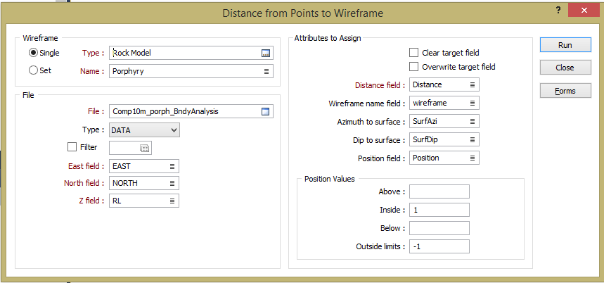Figure 2. The Distance to wireframes form allows you to flag your composites with distance to wireframe and the position of the point in 3D space with respect to the wireframe surface.

Once you run the form you have a fully flagged table that you can export to excel and complete the evaluation as per my Leapfrog examples (closely matching the LF Geo workflow in excel). You can however do everything in Micromine. First you calculate the positive and negative distances by simply running a calculation on the file to calculate positive and negative distances (File -> Fields -> Calculate), it is a simple calculation of WF_Distance = Distance multiplied by position (Figure 3). This gives you a good way of displaying the data and validating the calculation, is it doing what you expect it to (Figure 4)?


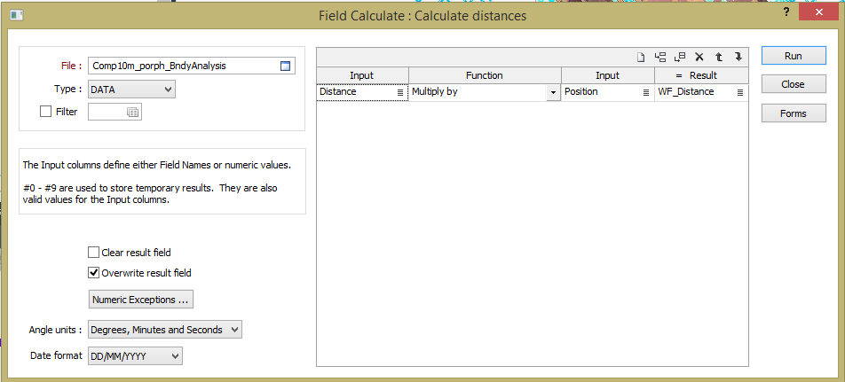Figure 3. A simple field calculation gives us the positive and negative distances needed for the calculations.


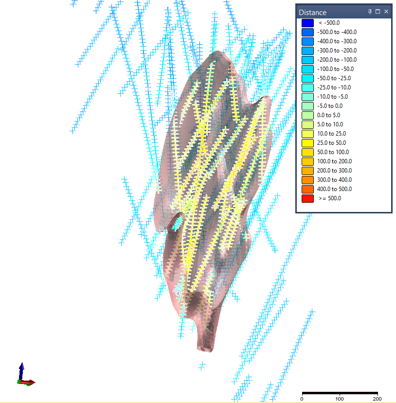Figure 4. Composites coloured by calculated distance from wireframe.

You then need to classify the distances into the relevant bins in order to assess the statistics. Because I am looking to run an estimate into 40m blocks I have composited to 10m (which is also a multiple of all my sample lengths), the best bin size to work with in this case is around 20m (half the block size). Some practitioners will want to test the boundary at a very detailed level - say 1m in this example. In my opinion this is far too detailed for the level of information we have. If we are estimating into 40m blocks we are doing so because of the spacing of our informing points and we will want to know what the contact looks like at our block size (or half block size). It may appear to be hard at 1m but at the size of the block it is soft - so that is really how it should be treated. If it is actually hard at 1 or 2 blocks distant then the boundary is hard for our purposes. Thus for this example I am going to classify my data into bins of  20m which will give me 2 "data points" for each block. I can do this using the File -> Fields -> Generate option (Figure 5).


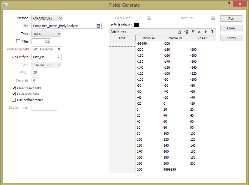Figure 5. The Fields Generate form - this allows you to classify the distances into Bins for further analysis - here I am using Bins of 20m because my blocks are 40m in size, I leave the bins more than 200m away blank as I am not really interested in this data and at these distances the points start to be influenced by other mineralised bodies and 200m will give me 5 blocks or 10 points of information either side of the contact which should be enough.

This process then flags each sample with a Bin ID, to do this the Wireframe distance field must be numeric - if it is character you cannot select minimum and maximum totals so select to modify the file and check. While you are in the file modify section you have to add a field to the table (call it number/sample number/ Number of Bins - whatever you like as long as it is meaningful) and then fill this with 1 (Thanks to Dave Bartlett from Micromine Support for helping me see this simple solution for a sample count and helping me with the final steps of this process).  Then you must sort the file by your new bin field (I sort by the bins first and then WF_Distance second just to be pedantic).

With the composite table flagged with distances, classified into bins and sorted by those bins we can then do a drillhole extract where we extract the data within each bin average it. If you have a Hole_ID and a depth from and depth to field Micromine will do this extract on a drillhole by drillhole basis when sorted by drillhole and drillhole depth but it still gives us a result we can use, more about this later. If you sort the table by the Bins field first (ascending from negative to positive) the extract will work on the bins only. Go to Drillhole -> Calculations -> Extraction and fill the form as indicated in Figure 6. This will average the assays and sum up the sample count for each bin (and by keeping the file sorted by the HoleID, From and To - each hole if you want that option). 


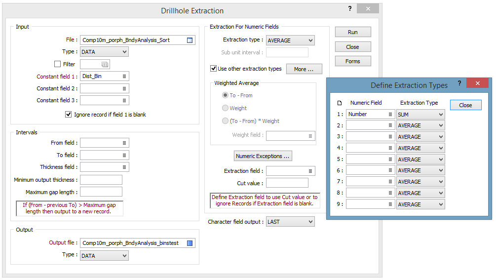Figure 6. Drillhole Extraction form, My constant field is the distance Bin. I have selected to average the assay fields but I want a count of the number of samples so I need to sum the sample count field I created earlier.

We now have 2 or 3 point files - one complete composite file which is flagged with all distance and direction from the wireframe in question which can be graphed, analysed and pulled apart. The information in the main composite file is not only useful for generating the Contact analysis but allows you to visually assess what is informing each individual composite and its impact overall. Another file that has been composed into distance bins with a sample count for each hole (if you have kept the file sorted by HoleID, From and To fields in the composite table prior to running the extract) which can also be analysed, pulled apart and assessed, with the bins already done it is an easier process to average the data in each bin using Excel and a pivot table. The pivot table gives you a simple way of grouping the distance data, the average grades and the sample counts into a format that you can graph (Figure 7), and a nice tabular representation of the jump in grade of it is there. 


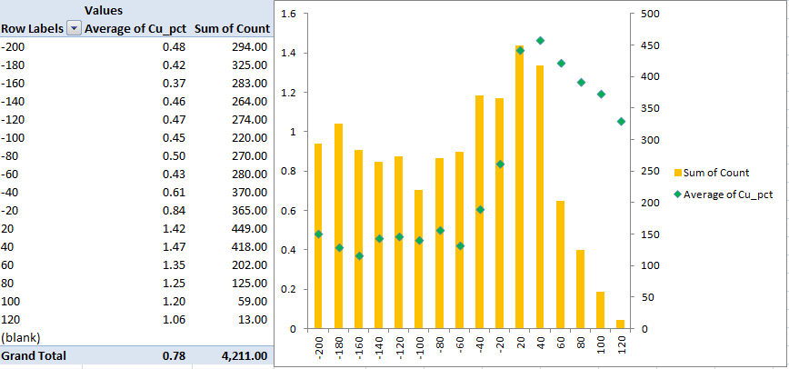Figure 7. Displaying the data as a Pivot Table.

There are a number of ways we can analyse all this data. First of all you can create a basic scatter plot of grade by distance using either the full composited file or the reduced binned by drillhole file, I generally use the full file as this allows more detailed analysis of the data through synced windows but it does have the affect of masking the boundary a tad as it contains a significant amount of data that can deceive the uninformed eye (Figure 8). These sorts of plots are very good at keeping us honest, when looking at a plot that contains a single point per bin (Figure 7) it is very easy to believe that there is no scatter behind it - seeing such a significant jump in grade in this plot helps convince you that the final contact analysis is probably correct.


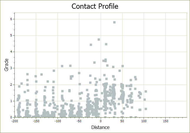Figure 8. Basic contact profile that plots distance against grade, whilst noisier than a traditional contact profile it does show the sort of scatter you would expect to see in reality and an average line through the data either side of 0m Distance indicates that a significant change occurs.

In Figure 9 I have specifically selected one composite, interrogated the dip, azimuth and distance from the wireframe and then created a string file using that information to see what part of the wireframe is informing this point. Very useful when you notice some anomalies in the data and which to find the cause.


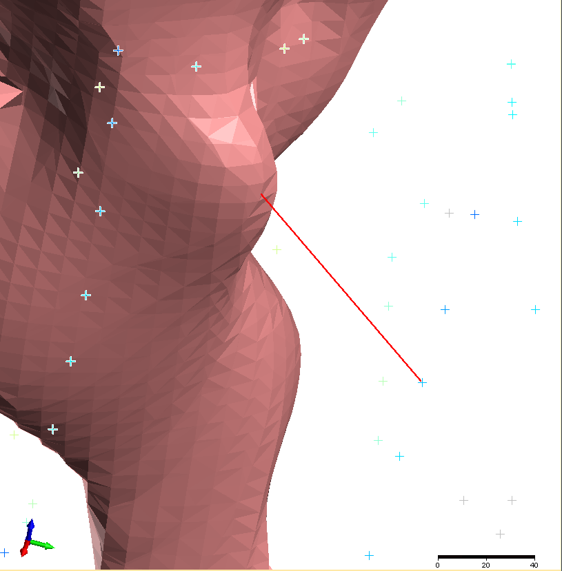Figure 9. Here I have used the Distance, SurfDip and SurfAzi information in the composite table to identify the exact portion of the wireframe that informs this particular point, remember the information is "From" the wirefame so to key in the correct coordinates you must reverse the Azi (+/-180) and Dip angles.

In Figure 10 I have generated some plots from the data and as the various windows have been synced I can click on something in one window and assess the location and impact of this on the analysis. In this case there is a anomalous population of data that sits in the -10 to -30 degree dip window of the histogram, selecting these two bars highlights the data in the stereonet, the main Visex view and the contact profile plot. I can see that there is a spread of the data both internal to and external to the porphyry wireframe and that while the grades inside the porphyry (Positive distances) are about average for the porphyry the points external to and on the south-eastern side of the porphyry are generally lower in grade than the rest of the dataset which might be important. You could also select all the data above a particular grade and assess the distribution - for instance are all the higher grades in a particular area and do they need to be domained out?


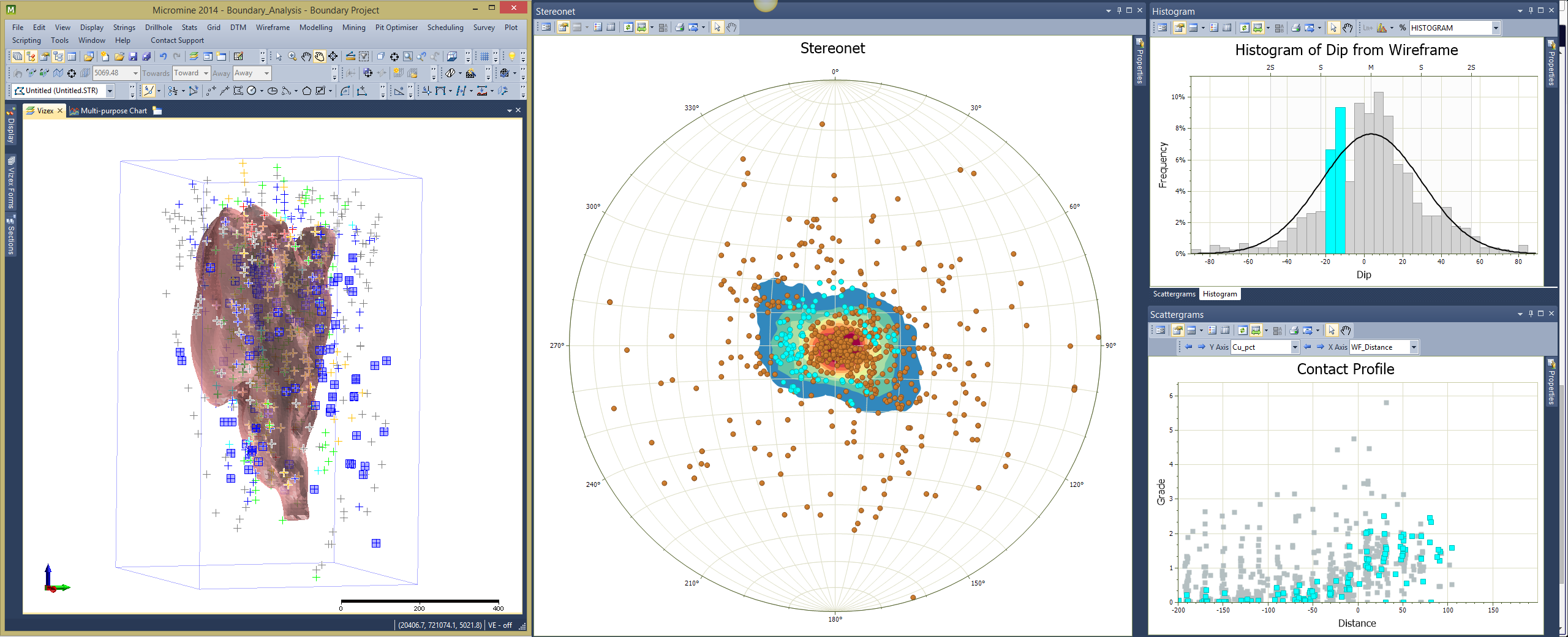Figure 10. With the various windows linked and the data at hand you can interrogate your data and assess the impact of various populations in the dataset - here for instance there is a prevalence of data in the -10 to -30 degree dip that is biased towards the eastern side. While it does not appear to have an effect on the contact profile analysis internally it does appear to be low on the external dataset.

At this point the composite file can exported from Micromine into a spreadsheet program such as Microsoft Excel. The data is then classified into bins of distance from the structure based on the surface interpolant and the mean grade of each bin calculated exactly as I have previously discussed for Leapfrog in the earlier blog posts. Whilst ideally this would be a declustered mean, a naïve mean is sufficient for our purposes unless the data is significantly clustered - it might then pay to decluster the data. These values are then graphed as a histogram and line graph (Figure 11). 


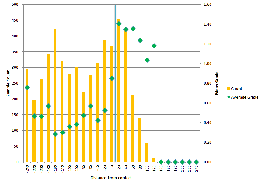Figure 11. The final contact analysis chart from Excel shows that a significant jump in grade occurs at the contact. We can see that once we exit the porphyry there is a significant fall in grade till the external grade is less than half the internal grade at 1/2 a block from the contact. It is quite evident that from the point of view of a block model this is a hard boundary.

However, if you have sorted the composite table by bin prior to running the drillhole extraction you will have a new table where all the information is divided into the relevant distance bins only, with a sample count and averaged grades. With this table there is no need to go external to a spreadsheet program as you can use Micromine's Multi-Purpose Chart option to graph up the results (Figure 12).


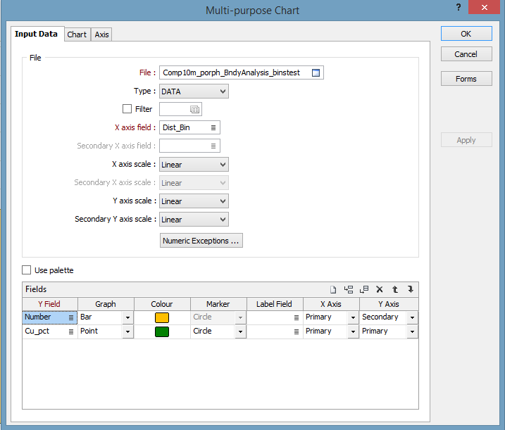Figure 12. Setting up a Contact Profile Chart in Micromine.

The results are then plotted as a chart that shows the sample count and the average grade per bin. Figure 13 shows the copper with a hard boundary, whereas Figure 14 shows the molybdenum chart, clearly this is a soft boundary with the Moly showing no real change across the contact.


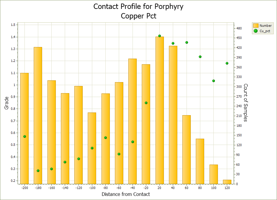Figure 13. The same contact profile as in Figure 7 but done in Micromine, clearly a hard boundary with over 0.5%  jump in Copper across the contact.


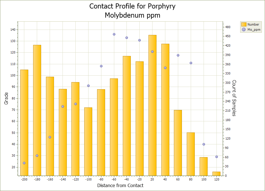Figure 14. Here we have a Molybdenum chart - clearly here the porphyry contact means next to nothing, just another rock Mo is passing through.

Repeating this analysis over several areas of interest will give a good indication of a realistic search strategy and Boundary condition. Large areas can be done rapidly, well within an hour. In this example I have used a thrust and oxidation contact to constrain and assess a lithological contact, the same process can be conducted on any boundary in the dataset, structural boundaries, alteration fronts, oxidation layers etc, very rapidly and with confidence. If your composite file has all your metals of interest to start with then you have everything at hand to rapidly test all your commodities.

While a number of programs will do a boundary analysis they are most commonly done along a drillhole by averaging the distances along the drillhole from a specific contact. When your drilling is normal to the contact this is perfectly reasonable and gives good results. Generally in the mining industry this is not the case and the effect of this sort of analysis on drillholes that are at a high angle to the contact will always result in a smoothed un-representative graph that cause the contact to appear soft when this is not the case. There are some programs that you can purchase through various consultancies that attempt to measure the distance from a point to a wireframe but having never used these I cannot comment on their accuracy.  However, if you own a Micromine licence (or Leapfrog) you have access to a robust and accurate method of conducting a boundary analysis, and the beauty of Micromine is it is all internal - no reason to go external to another program just to complete you analysis.

Happy Modelling!