This is a series of posts written by mineral industry technical leaders, and first off the block is Ron Reid of Harmony Gold SE Asia.  Ron's expertise in Leapfrog began from a Leapfrog training workshop that I ran at Harmony Gold and now Ron is the resident expert of Leapfrog within Harmony Gold SE Asia.  This post is an example of very practical instructional material that we would save as white papers in the restricted area for registered users.  Today we are making this material available to all visitors to the website. Many thanks for your contribution, Ron! - Jun Cowan

---

Domain boundaries - hard or soft?

Anyone involved in resource estimation has been faced with the decision of how to treat a domain boundary. There are several issues that need addressing:

• Should it be treated as a hard boundary i.e. one that is opaque to data either side of the boundary?
• Should it be treated as a soft boundary, one that allows data to be seen across it, and if so, for how far into the domain?
• Should it be treated as a one way or a two way domain boundary? 

Careful assessment of the data will allow an estimator to make this decision by visual assessment; however, in this day and age we are commonly required to “prove” our decisions.

Some general mining packages (GMP) allow a composite file to be flagged with the distance from a contact to allow a profile to be plotted, but what to do if we do not have access to these packages. Those of us who have access to Leapfrog Mining have a ready platform with which to analyse a boundary and make a quantified assessment of whether a boundary is hard or soft. Take the dataset shown in Figure 1. This dataset is part of a porphyry copper deposit and shows that the deposit is cut by a significant thrust that appears to offset the hangingwall by some 250m. 
   



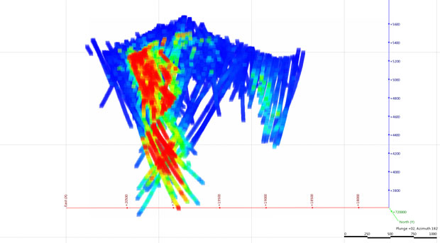
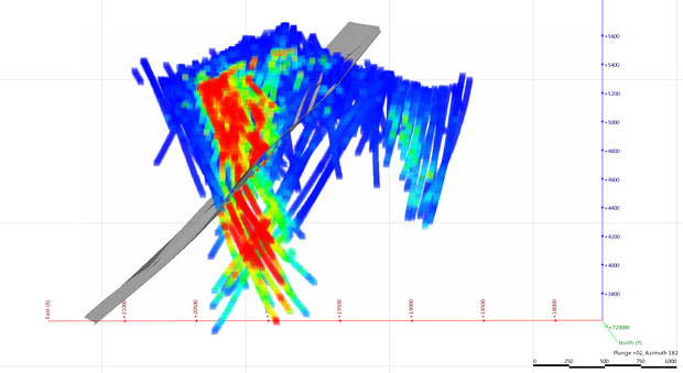Figure 1. Identify the relevant structure - here the copper mineralisation appears to be cut by a thrust. On the right a thrust has been modelled; in this case the thrust is a known structure and has been related back to faults observed in core photos.

The first requirement is to identify and then model the fault zone as shown in Figure 1. With access to the original core photos, field mapping and structural mapping this process becomes a basic structural geology problem, else you can use Leapfrog to model it in where you believe it to be located.


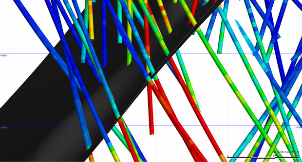Figure 2. Visual assessment shows a very strong break in grade - visually the boundary appears hard, the thrust could be used to define a domain boundary.

At this point basic visual observation will show that the contact should be treated as hard (Figure 2).  How do we show this in a statistical / graphical form to satisfy those that will ask for “a full boundary analysis”? The ability in Leapfrog 3D to create domains, data subsets and evaluate the composites against this data creates an opportunity to accomplish just that.

If we were to assess the global dataset against the thrust modelled in Figure 1 we would get ambiguous results due mixing the various domains. To obtain a more accurate picture we must subset the data. To do this we select a section of the boundary with sufficient data density to assess what happens to the grade across the boundary. A domain is generated that covers the area of interest and is used to subset the composite file into localised data around the boundary. As the thrust in the example was digitised using polylines we need to export the surface wireframe and re-import the points as a boundary data type to allow a distance interpolant to be calculated. There are two ways to do this, new versions allow you to right click on the mesh boundary and “Extract mesh vertices”, else you can export and re-import the mesh. Exporting the surface as a Micromine Pnt and Tri asci file (or equivalent Datamine files) is a simple way of doing this as the point file is then easily re-imported as a Boundary point file. Once converted to a boundary file the surface is then re-created as a surface interpolant and a distance interpolant is also calculated. I generally only create the surface and interpolant within the domain I am evaluating – no point in creating an additional large layer if not needed (Figure 3).


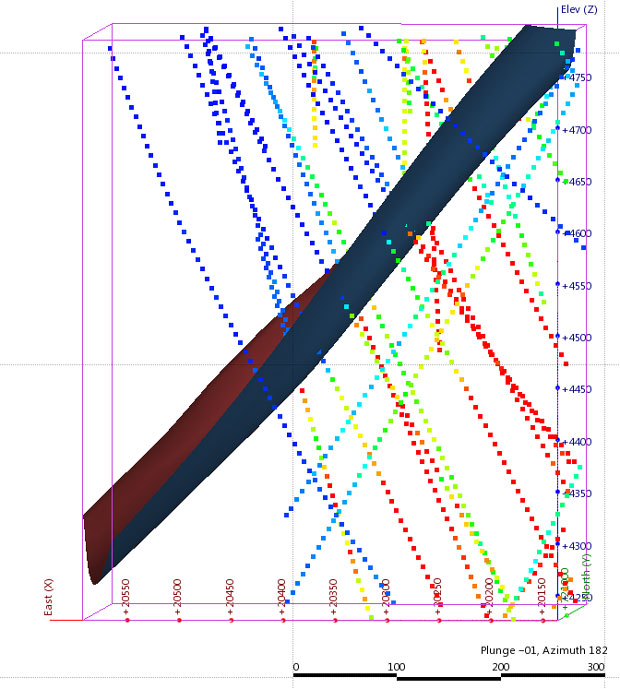Figure 3. A domain is generated to select out a specific area of composites to test the contact locally (here coloured by grade).


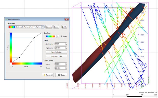
Figure 4. A distance interpolant is generated on the contact to allow the composites to be accurately evaluated for distance from the thrust. Note there are two drillholes that drill parallel to the thrust, these may cause an issue with the analysis and is something to keep in mind.


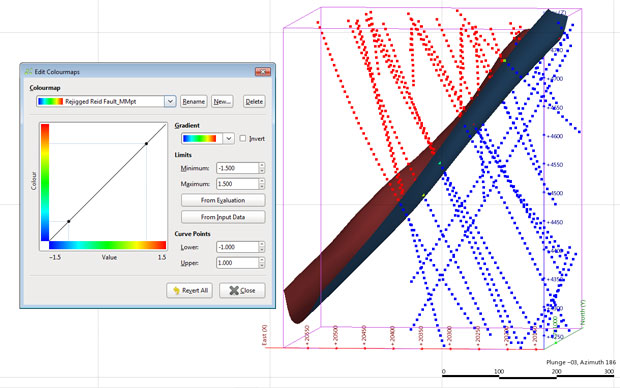
Figure 5. The composites are also evaluated against the thrust itself to allow us to determine upper and lower domains within the composites, note the hanging wall is positive (red) and the footwall negative (blue).

At this point we can evaluate our subset composite file against the fault. We evaluate both the distance interpolant (Figure 4) and the surface interpolant (Figure 5). The distance interpolant lets us evaluate the linear distance from the fault, whereas the surface interpolant will give us a positive and negative quasi distance either side of the fault. This distance is not a true distance so cannot always be used to determine distance for a resource estimation search strategy, the distance interpolant allows an accurate distance to be calculated.

The composite file is then exported from Leapfrog and opened into a spreadsheet program such as Microsoft Excel. The data is then classified into bins of distance from the structure based on the surface interpolant and the mean grade of each bin calculated. Whilst ideally this would be a declustered mean, a naïve mean is sufficient for our purposes. These values are then graphed as a histogram and line graph (Figure 6).


Figure 6. The average grades of the composites are plotted up against the surface interpolant. The red and blue horizontal lines indicate the approximate population mean above and below the fault. Several composites that appear irregular are circled and require more analysis.

Figure 6 shows the footwall on the left (the negative side of the thrust) and the hanging (positive) side on the right. It appears that there are some irregular composites in the data between -80 and -40 units from the fault. We can filter the composites in Leapfrog3D using the surface interpolant evaluation.


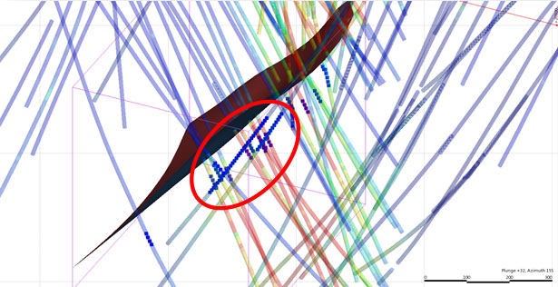Figure 7. Filtering the composites (dark blue) by the thrust evaluation for the affected distance shows as feared earlier, two drillholes (co-incident with the edge of the mineralisation)are drilled parralel to the fault and are responsible for the irregular lower grade composites in Figure 6.

Figure 7 shows that the two drillholes raised as a concern earlier lie within this distance from the structure. Analysis indicates that these holes sit just outside the mineralised domain and the long lengths of low grade is causing the low mean issue seen in the footwall (Figure 6).
 
The two drillholes are filtered from the data and the data reassessed, Figure 8 shows the results.


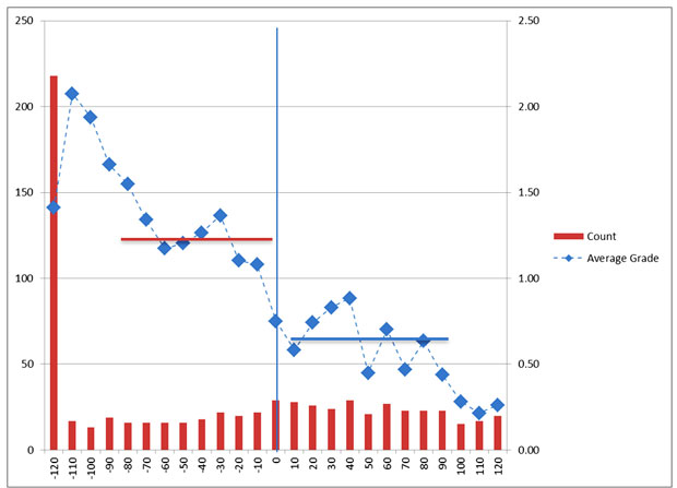Figure 8. Filtering the two anomalous drillholes out of the database cleans up the data so that a more accurate assessment of the data can be made. The red and blue bars indicate the mean location for the data out to a reasonable distance from the contact. The analysis indicates a hard boundary should be considered for resource estimation.


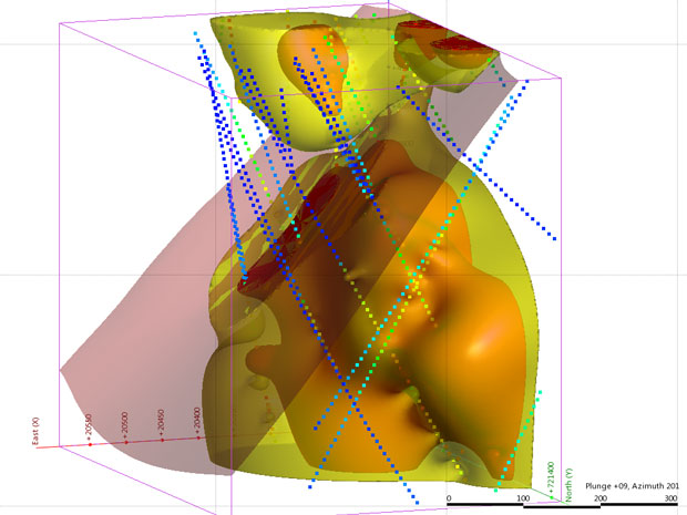Figure 9. The composites above and below the fault have been interpolated indiviually based on the boundary analysis. This shows a simple isotropic model over only a small portion of the overall project but clearly shows the affect of the thrust on the grade distribution in the deposit.

A significant increase in grade on the footwall side of thrust indicates that this contact is a hard boundary and should be treated as such in the estimation process. This information can be used in several modelling processes:

• To generate a grade model in Leapfrog Mining (Figure 9)
• To flag domains within a Grid of Points in Leapfrog that can be exported to a GMP as a flagged and evaluated block model
• Used externally in utilising a GMP to create a classic block model.

Repeating this analysis over several areas of interest will give a good indication of a realistic search strategy and can be done rapidly within an hour or two. In this example I have used a thrust, the same process can be conducted on any boundary in the dataset, lithological boundaries, alteration fronts, oxidation layers etc.

Ron Reid
Group Resource Geologist
Harmony Gold SE Asia Pty Ltd.