In my last post I mentioned that I composite for basic geostatistical reasons. Recently I observed a Leapfrog grade interpolation run on raw gold assays, using a linear variogram, and the result was awful to say the least and in fact was completely wrong by any measure. From a geostatistical point of view a number of rules were broken, it is not the purpose of this article to go into these in detail, but rather show how a simple application of some basic rules of thumb will result in a much more robust grade model. Here I will cover the basics of the database, compositing, applying a top cut, approximating a variogram and the basics of finding a "natural" cut for your first grade shell in order to define a grade domain to contain your model.
Note that in the forthcoming discussion I refer largely to processes in Leapfrog Mining, it being a more powerful and useful tool than Leapfrog Geo in its current form, however if you are a Geo user the following still applies – the workflow may be slightly different.
The database
As in all things the GIGO principle, "garbage in, garbage out", applies in Leapfrog. If your database has not been properly cleaned and validated you will get erroneous results. I have noticed that many LF users will load a drill hole database and not fix the errors flagged by Leapfrog. The most common issue is retaining the below detection values as negative values such as -0.01 for below detection gold for instance. If this is left in the database then the interpolation will use this value as an assay and it will lead to errors in the interpolation model. It is better to flag it as a below detection sample and instruct Leapfrog in how to treat these. Where the database uses values such as -9999 for lost sample, or -5555 for insufficient sample you will get a spectacular fail when you attempt to model this (yes it does happen!). If you only have a few errors it is simple enough to add a few special values through the fix errors option to correct these issues (Figure 1). If you have a large number of errors the fastest way to fix the errors is to load the data once, export the errors in order to identify them and then build a special values table that records each error. This is fairly simple to do and should be laid out as shown in Figure 2, you save this as a csv into the same folder as your drill hole data. This file can then be used for every LF Mining project you build as long as your field names do not change, or the particular assays do not vary, although it is not too big a job to adjust the table if need be. You then delete your database from your project and reload it, selecting the special values table at the same time (Figure 3), the database will then load with the assay issue fixed. If you are a Leapfrog Geo user you cannot do this as the special values option has been removed, you have to manually correct and validate as assessed every error flagged (a process that can become quite tedious in a large project, and frustrating; Figure 4). Once your assay table has been validated you can move on; technically your whole database should be validated but I will take it as a given that the process has been completed, most people understand issues around drill holes with incorrect coordinates or drill holes that do a right hand bend due to poor quality survey data.
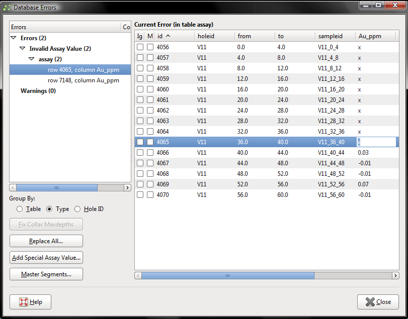
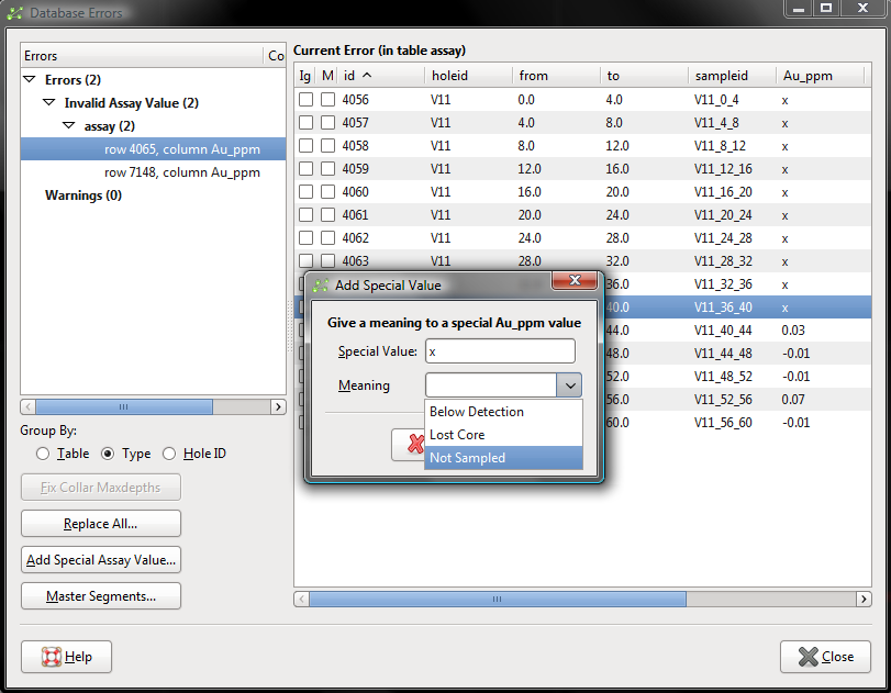
Figure 1. Fixing a simple series of errors in Leapfrog Mining is a simple process as the file can be adjusted to correct errors. In this case I have 2 errors, a series of X’s that represent insufficient sample, and -0.01 which is below detection. I can fix these using the Add Special Assay value… option and selecting Not Sampled or Below Detection.

Figure 2. With Leapfrog Mining you can create a Special Values Table that can be loaded at the Database import stage, the Special Values Table should be structured as above.
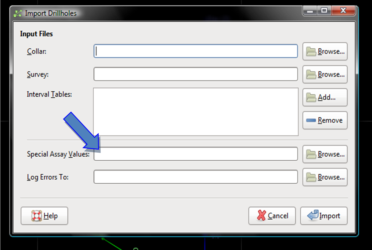
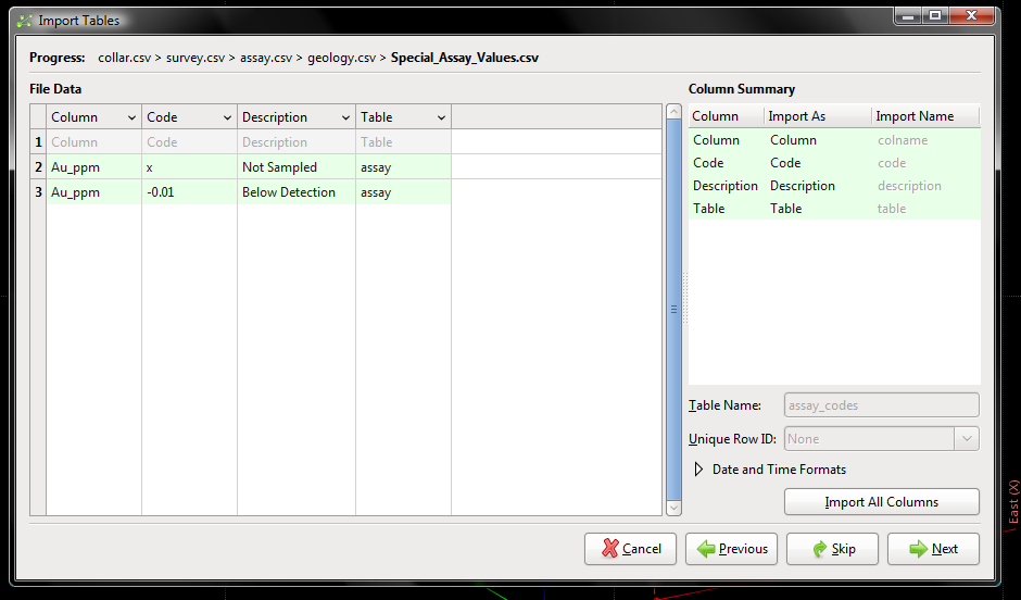
Figure 3. Top image shows where you can load the Special Values table (blue arrow), this can only be loaded at the time of loading the database, it cannot be added after the database has been loaded.

Figure 4. Leapfrog Geo does not have a facility to import Special Assay Values, you must manually correct the errors every time you create a new project, once the rules have been decided you must tick the “These rules have been reviewed” option to get rid of the red cross.
Composite your data!
I have not yet come across a drill hole database that consists of regular 1, 2 or 3 metre sampling, there is always a spread of sample lengths, occasionally due to sampling on geological boundaries, through to bulk background composites and un-sampled lengths. This leads to a large variation in what is termed support length (Figure 5). It is also common for there to be a correlation between sample length and grade, ie smaller sample lengths where grade is higher (Figure 5). This can lead to problems with the estimation process that is well understood in Geostats, perhaps less well understood outside of the resource geology world. Leapfrog's estimation is basically a method of kriging, and so is subject to all the foibles of any kriged estimate, these include issues of excessive smoothing and grade blow outs in poorly controlled areas. Leapfrog has a basic blog article about how leapfrog’s modeling method works on their website. Having multiple small high grade intervals and fewer larger low grade intervals will cause the high grade to be spread around (share and share alike!).
A simple way of dealing with this is to composite your data. Compositing has a dual effect, it regularises your sample support and also acts as a first step in reducing your sample variance (Table 1). It effectively "top cuts" your data by diluting the very high grades. Now there are two sides to the top cut-composite order fence. Those who swear you top cut first, those that say neigh, top cut is always applied after the composite. I am going to declare a conflict of interest in that I sit in the TC post composite camp, for pure practical reasons as I will explain below.
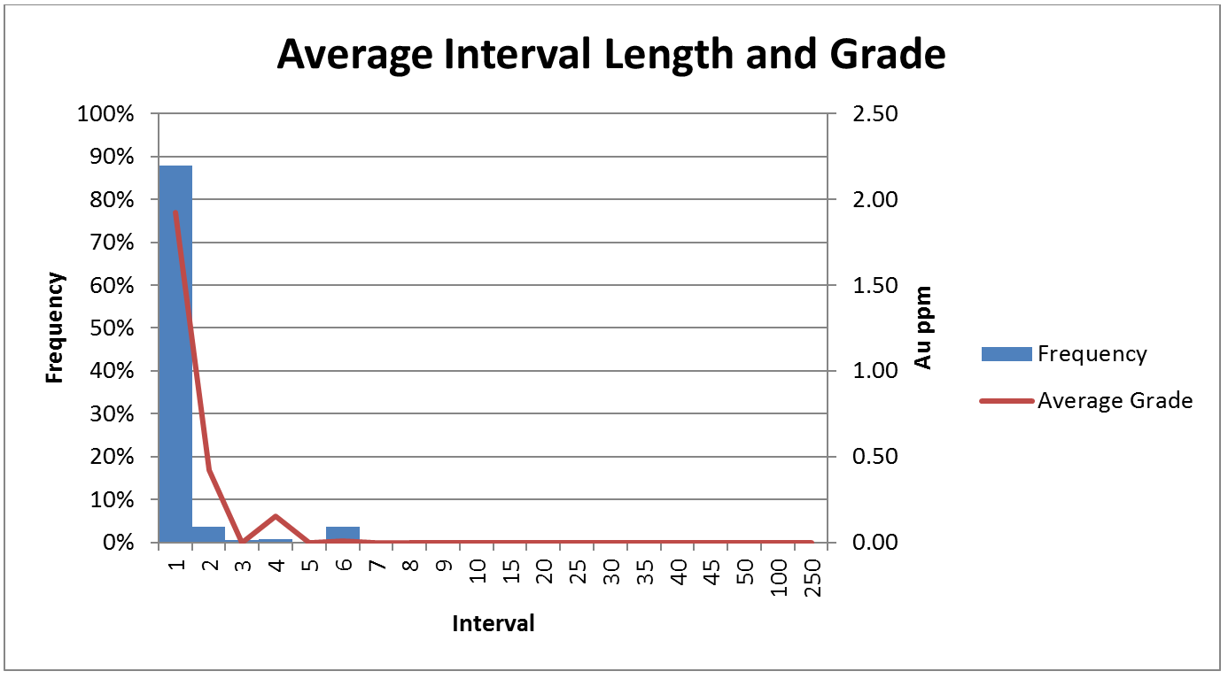
Figure 5. Graph showing sample interval length with average grade by bin, it is evident that the 1 and 2m intervals have significant grade and should not be split by compositing, bin 4 only has minor grade and bin 6 has no grade, it is probably not a significant issue if these bins are split by compositing. I would probably composite to 4m in this case as the 4m assay data may still be significant even if the number is not high (and I happen to know the dataset is for an open pit with benches on this order), 2m would also be a possibility that would not be incorrect.
With respect to the regularising of the sample length, this has a profound effect on the variability of the samples and will also give you a more robust and faster estimate. Selecting a composite length can be as involved as you want to make it however there are a couple of rules of thumb; first your composite length should relate to the type of deposit you have and the ultimate mining method, a high grade underground mine will require a different more selective sample length to a bulk low grade open pit operation for example. The other rule of thumb is that you should not "split" samples, ie if most of your samples are 2m, selecting a 1m or even a 5m composite will split a lot of samples, spreading the same grade above and below a composite boundary, this gives you a dataset with drastically lower variance than reality (which translates as a very low nugget in the variogram), and results in a poor estimate. If you have 2m samples you should composite at 2, 4 or 6m, if you have quite a few 4m samples then this should be pushed out to 8m if 4m is determined to be too small, the composite should always be a multiple of those below it. This must be balanced against the original intent of the model and practicality, it is no good using 8m composites if your orebody is only 6m wide, and the longer the composite the smoother the estimate and you are creating the same issue you are trying to avoid by not splitting samples. You will find that there is commonly very little change in the basic statistics once you get past 4-6m, and implies that there is no real reason to go larger from a purely stats point of view, there may be however from a practical point of view.
For the sake of the argument here let us assume a 5 metre composite will suit our requirements. Having assessed our raw data we find that we have a data set that has extreme grades that imply the requirement for a top cut of say 25gpt gold (I will stick to gold in this discussion but the principle applies across the board), the question becomes "should I composite pre or post applying the top cut?”. Let’s say the 1m samples that make up a particular composite are 2.5, 5.8, 1.6, 125.1, and 18gpt. The straight average of this composite would be 30.6 gpt. If I apply the top cut first I would get 2.5, 5.8, 1.6, 25.0 and 18gpt which will composite to 10.58 gpt gold. If I apply the top cut after, my grade for the composite will be 25gpt (given the original composite grade is 30.6 cut to 25). As you can see by applying the top cut first we are potentially wiping a significant amount of metal from the system, also when assessing the dataset post-composite it is sometimes the case that a dataset that required top cutting pre-compositing no longer requires it post, or that a very different top cut is required – sometimes a higher one than indicated in the raw dataset. If geological sampling has been done where sample lengths are all over the shop this becomes even more involved as length weighting has to be involved. Besides, it is a simple process to top cut post-compositing in Leapfrog which makes the decision easy (Figure 6). Why do we top cut in the first place you might ask, simply because if we were to use the data with the very high grade (say the 125.1 gpt sample above) we will find that the very high grades will unduly influence the estimate and give you an overly optimistic grade interpolation.
Applying a top cut in leapfrog is a simple process of assessing the data in the histogram (Figure 6); Table 1 shows the statistics for the gold dataset shown in Figure 5 and Figure 6, composited by lengths of 2 and 4m. Statistical purists will say the CV values presented here are too high for a kriged estimate, true from a geostats point of view but this is a real dataset and sometimes we have to play the hand we are dealt, we are not trying to generate a Stock exchange reportable estimate so do not get too caught up in this argument.
Note that you cannot currently create a composite file prior to creating an interpolant in LF Geo, you must create an interpolant and shells first, specifying a composite length, prior to analysing the composited datasets.
Table 1. Statistics of raw data for a WA lode Gold deposit, showing the effects of compositing and applying a top cut to the composite table.

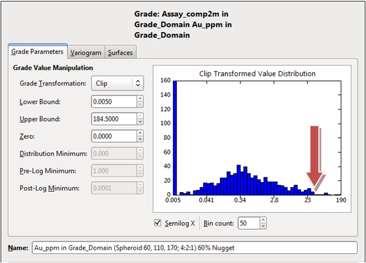
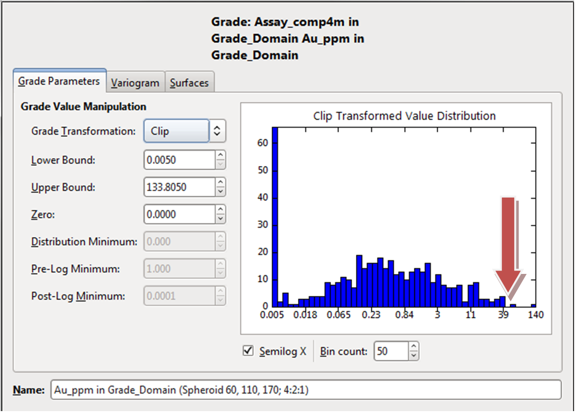
Figure 6. You can pick a simple top cut that stands up to relatively rigorous scrutiny using the graph option when generating the interpolant. A widely used method is to select where the histogram breaks down, this at its most basic is where the histogram starts to get gaps, here it is approximately 25g/t for the 2m dataset on left but 40g/t for the 4m Dataset on right (arrowed in red, lognormal graph is simply for better definition), you enter this value into the Upper Bound field to apply the top cut.
The Variogram
Never run a grade interpolation using a linear variogram, doing so implies that two samples, no matter how far apart, have a direct linear relationship, which is never true in reality and can lead to some very weird results (Figure 7). A basic understanding of sample relationships is essential when running a grade interpolation. Namely that there is always some form of nugget effect, ie two samples side by side will show some difference, and that as you move the samples further apart the samples lose any relationship to each other so that at some point the samples bear no relationship to each other. In cases where two samples side by side bear no relationship at all we have a phenomenon known as pure nugget, in this case you may as well take an average of the whole dataset as it is neigh impossible to estimate a pure nugget deposit, as many companies have found to their cost.


Figure 7. This figure shows the effect of applying a linear isotropic variogram (blue) and a spheroidal 50% nugget variogram (yellow) to the same dataset, each surface represents a 0.3g/t shell, a significant blow out is evident in the Linear variogram.
Given that one benefit of Leapfrog is its ability to rapidly assess a deposit, it does not make sense to delve deeply into a geostatical study of sample distribution and generate complex variograms, especially given Leapfrogs simplistic variogram tools. However a basic understanding of how a variogram should behave for various deposit types will allow you to approximate the variogram for your dataset. For instance, the nugget value for most deposits (assuming few sample errors) will generally be the same across the world, a porphyry gold deposit will have a nugget somewhere between 10-20% of the total variance (call it 15%), epithermal gold deposits tend to sit in the 30-60% range (call it 40%) and lode gold deposits are commonly in the 50-70% range (call it 60%). Changing the Nugget can have a significant effect on the outcome (Figure 8). Ranges are the inverse to this, generally the smaller the nugget the longer the range, a porphyry deposit for example may have a 450m range, whereas a lode gold deposit may only have a 25m range. The Alpha variable controls the shoulder of the variogram, a higher number will give you a sharper shoulder (Figure 9), this is also related to the deposit, a porphyry deposit might have a shallower shoulder and thus an alpha value of say 3, whereas the lode gold deposit may have a very sharp shoulder and thus an alpha value of 9 maybe more appropriate. The alpha values are also useful if you know your variogram has several structures, if you have several structures a lower alpha number helps approximate this. Beware if you are a leapfrog Geo user this relationship is the reverse – changes to the way Leapfrog Geo works means that a LF Geo Alpha 3 = a LF Mining Alpha 9 – software engineers just like to keep us on our toes!
Let us say we have a lode gold deposit, we will assume a nugget of 60% of the sill, a range of say 25m and use an alpha value of 9.
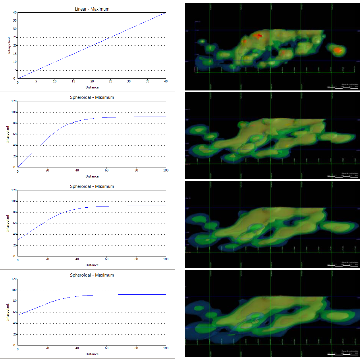
Figure 8. Figure showing the effect of varying the nugget value, Top is a straight isotropic linear interpolation (Linear is always a No No), below that is a 0% nugget, then a 30% nugget and finally a 60% nugget.
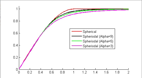

Figure 9. Figure showing the effect of the Alpha Variable, on the graph on the top is for LF Mining, the graph on the botom is for LF Geo; Note that the variable changes between Mining and Geo so that a higher Alpha variable in Mining (eg 9) is equivalent to a low Alpha in Geo (eg 3).
The "natural cut"
The next step is to define the natural cut of the data. Sometimes when we run an interpolation we find that the lowest cut-off we use creates a solid box within our domain (Figure 10), this is because there are too many samples at that grade that are unconstrained, ie we are defining a background value. The first step in defining a set of shells from our interpolant is to start with one low grade shell, say 0.2gpt. As we are creating just one shell, after the interpolant has been created the one shell is quite quick to generate. We may find that 0.2 fills our domain so generate a shell of 0.3 and re-run, continue doing this until you find the cut-off where you suddenly switch from filling the domain to defining a grade shell, this is your natural cut-off for your data (Figure 10). You can use this as the first shell in your dataset, simply add several more at relevant cut-offs for assessment and viewing, or you can generate a Grade Domain using this cutoff to constrain an additional interpolation that you can then use to select and evaluate a grid of points, effectively generating a Leapfrog block model.
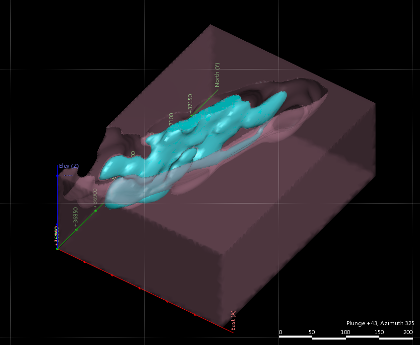
Figure 10. Figure showing the effect of shells above and below a natural cut-off. Brown = 0.2g/t which is an unconstrained shell, blue=0.3g/t which is the constrained shell and defines the natural cut-off of the dataset.
Following this process outlined above will vastly improve your grade modelling and lead to better interpolations with better outcomes. Note I have not spoken about search ellipses, major, minor or semi minor axis, orientations of grade etc, this is because this is all dependent upon the deposit. Your deposit may require an isotopic search, or some long cigar-shaped search, depending upon the structural, lithological and geochemical controls acting upon the deposit at the time of formation and effects post formation. The average nugget and the range of the variogram will generally conform to what is common to that deposit type around the world. A bit of study and research on the deposit is something that should already have been done as part of the exploration process, adding a quick assessment of common variogram parameters is not an arduous addition to this process. It is not a requirement to understand the intricacies of variogram modelling, nor the maths behind it, but knowing the average nugget percent and range for the deposit type should be an integral part of your investigations, and should inform your Leapfrog Grade interpolations.
Happy modeling…