This is an article by Paul Hooykaas which was recently
published by Micromine. The article is reproduced in full. At a later date, Orefind will be putting up posts about the definition of
implicit modelling, so I'm calling this
Part 1. - Jun Cowan
---
Introduction
It seems that everyone wants to jump onto the implicit modelling bandwagon.
The Orefind blog page reflects this trend, with at least six related articles since late 2012 – Jun Cowan and Ron Reid being the notable contributors.
Unfortunately it appears that the industry does not have a consistent understanding of the term “implicit modelling”. I say unfortunately, because the original definition is being compromised to the extent that reviewers now resort to saying “true implicit modelling”, when really the “true” qualifier should not be necessary.
So this is an attempt to clarify what implicit modelling really is. The term is a relative newcomer to the mineral resources sector, but the computer graphics industry has been using the underlying methods since the late 1960s. Consider this extract from Jules Bloomenthal’s thesis, Skeletal Design of Natural Forms (Jan 1995).
“Geometric modeling is often classified into parametric and implicit methods. Both are well developed in computer graphics (early parametric methods are described in [Coons 1967] and early implicit methods are described in [Mathematical Applications Group 1968]. Implicit surfaces more readily capture the volumetric relationship…”
In mathematics the word “implicit” has far longer history, and is used to describe a particular type of function.
Implicit or Explicit?
“Implicit Modelling” was introduced to the exploration and mining industry by Jun Cowan in a paper presented to the Fifth International Mining Geology Conference, held in Bendigo, November 2003. Much of this article reiterates the content of that paper.
Perhaps to emphasise the concepts associated with implicit modelling, the paper described traditional modelling methods (those relying heavily on manual digitising) as ‘explicit’. I believe this reference may have inadvertently caused some of the confusion we see today. In every day conversation the words ‘implicit’ and ‘explicit’ are antonyms (the former denoting “fully and clearly defined” and the latter “not directly expressed”). By associating both words with the modelling process, it suggests that every method must fall into one of these two categories. Since the explicit method was well understood, it was convenient to classify any procedure that generated a suitable output, but did not involve manual digitising, to be considered as “implicit”. For example, it is popular to claim that generating one or more grade shells, from a 3D block model, is a form of implicit modelling. Although this is clearly not an explicit technique, I suggest that it is not an implicit method either. This is not as odd as it seems once you realise that the ‘implicit’ descriptor came from a mathematical meaning, rather than common usage.
Curves and Surfaces
Much of the reference material for this topic refers to ‘curves’ and ‘surfaces’. It is worth discussing the mathematical definitions of curves and surfaces, because they differ slightly from the standard understanding of these terms:
- A curve is similar to a line but is not required to be straight. An open curve has beginning and end points that are different. A closed curve joins up, so there are no end points.
- Surprisingly the (geometric) definition of a surface can quickly become cluttered with technical terms like “manifold’ and ‘Euclidean’. A simple description is “part, or all, of the boundary of a solid”. The main point is that surfaces, like curves can be open or closed. A plane is a simple example of an open surface, and a sphere is a closed surface. Another way of looking at it is that an open surface has an area and a closed surface has a volume.
Function Types
So what does “implicit” mean in a maths context? In mathematics the relationship between x and y (for curves) or a relationship between x, y and z (for surfaces) are called functions and there are three distinct function types: explicit, implicit and parametric.
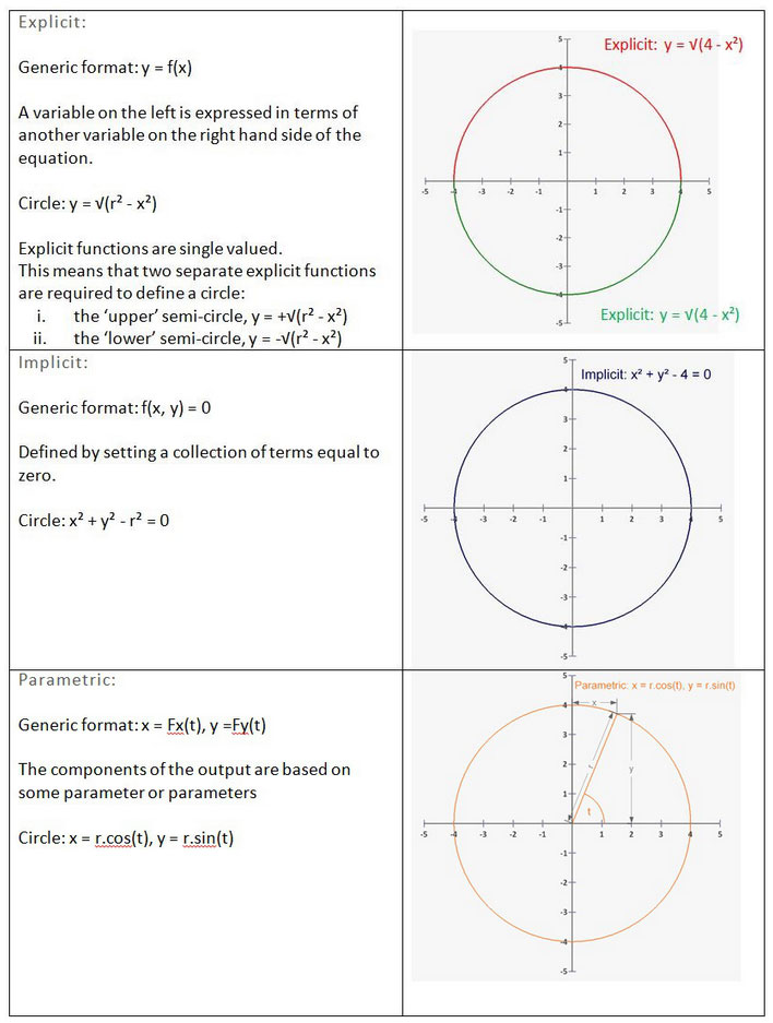
Using a circle, as an example, the three type are illustrated below. To keep things simple, the circle is centred at 0, 0 and has a radius = 2.

Notes:
- The above is based on a curve (or line) using variables x and y. We can extend the discussion to include surfaces by introducing a z variable.
- There is a subtle distinction between functions and equations, which has been ignored.
---
Explicit functions generate y values directly from x values, so generating a series of points that lie on the circle is relatively easy. However the single value restriction (closed lines, or surfaces, are not supported) makes the explicit form unsuitable for our purpose.
Implicit functions do have a connection with the common usage of the word “implicit”. Staying with our circle example, remember that the implicit function is x² + y² – r² = 0. Based on that, and given a specific radius (say 2), think about how you would draw the circle. There is no direct way to systematically generate consecutive points that lie on the circle, and this is why the representation is called implicit. We know the circle is there – it is certainly well defined – but representing it visually is problematic.
But the implicit form has its own special properties. For a particular circle (where the radius is a known value), we can substitute
any x, y into the equation. If the result is positive the point is outside the circle. If it is negative the point falls inside the circle. If the result is zero then the point lies on the circle. In other words we can easily determine the ‘classification’ for any point.
The Parametric representation, on the other hand, provides a very convenient way to draw the circle. Start with t = 0 calculate x and y. Now increment t by a small amount and calculate the next x, y values. Continue this process until t = 2π…
An Implicit Model
Consider a 3D volume, containing a variable, but measurable attribute. This ‘attribute’ might be density, temperature or the grade of an ore body. Actual measurements have been taken at scattered data points. The data points can be used to derive an implicit function providing a continuous mathematical representation of the attribute across the volume. This implicit model contains an infinite number of isosurfaces – surfaces representing points of a constant value. A grade shell is a familiar example of an isosurface.
But the implicit model, itself, cannot be visualised. To do so we must extract one or more isosurfaces from the model and then display these in 3D space. If the model could be converted to a parametric form, extracting an isosurface would be easy. But life is not meant to be simple, and finding an equivalent parametric solution is too much to hope for.
As we saw earlier, with our circle example, an implicit model has no direct way to systematically generate points that lie on an isosurface. It provides a test for determining whether a point is on the surface, above the surface or below the surface, but it does not give any explicit rules for generating the surface points themselves.
The Definition (finally)
An Implicit Model is a continuous mathematical representation of an attribute across a volume. It has an infinitely fine resolution. Creating tangible surfaces from this model is a separate and secondary step and is independent of the creation of the Implicit Model.
Let’s revisit the scenario of generating grade shells from a block model. This fails against the above definition on two counts. Firstly the model is a discrete set of points, each having an associated grade value, rather than being a continuous grade representation across three dimensional space. Secondly the resolution of the output surface is dependent on the size of the blocks in the original model.
Isosurface Extraction
Implicit modelling generally has distinct 3 parts:
- Organise the data into an appropriate format
- Generate a continuous, volumetric model (the implicit model)
- Output one or more surfaces contained in the model
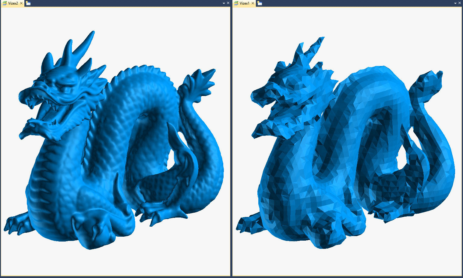
The output is almost always a triangulated mesh, or wireframe. Because triangles have straight sides the output wireframe is an approximation of the modelled surface. The finer the mesh (the smaller the triangles) the better the approximation, and the smoother the appearance. The mesh size is a compromise between a better fit and increased computing time.
Since there is no direct way of generating surface points, we must resort to indirect means. One of the most common methods is called “marching cubes”.

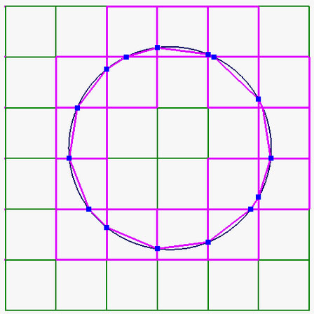
The principle can be (simplistically) illustrated by using “marching squares” in our 2D circle example. Starting with a square positioned in the top left corner of our extents, evaluate the implicit function for each corner of the square. If all corners return positive values, then the square is completely outside the circle. Equally, if all corners return negative values, then the square is completely inside the circle. If some corners are outside, and others are inside, then the square intersects the circle and we can calculate the line of intersection. If we covered the region with a grid of equal sized squares we would finish up with a set of line segments that approximate the circle. The smaller the squares, the larger the number of line segments and the smoother the result.
In a 3D context the size of the cube controls the resolution of the final surface. The two dragons, in the screenshots below, are based on the same underlying implicit model, but the surfaces were generated using a different mesh sizes.

Radial basis functions
Implicit modelling is invariably associated with Radial Basis Functions (RBF). These have been identified as one of the most accurate and stable methods of solving scattered data interpolation problems.
Basis functions have been described as mathematical Lego. They are a set of basic functional building blocks that can be stacked on top of one another to provide the features that we need.
Radial basis functions are a group of functions that generate values dependant on distance. So the closer you are to particular point, the more influence it has. The more common types are:
Gaussian
Multiquadric
Inverse quadratic
Inverse multiquadric
Polyharmonic spline
Similarly, Fourier Basis Functions are a group of functions related to waveforms…
Appealing to my survey background is a 2003 thesis by Grady Wright, who suggests that RBF development was initially (1968) developed in order to generate automated and unbiased contour maps.
Summary
I’ve recently been asking geologists and mining engineers what they think Implicit Modelling is. The answers have been variable and usually have an air of uncertainty. The resources industry has had exposure to this modelling technique for just over ten years now. But the methodology was adopted from geometrical processes that had been around for much longer. We must follow the mathematical trail to establish what is meant by implicit modelling. Once we do that, a clear definition is apparent. It is a continuous representation of a numeric attribute across a volume. The model is a mathematical function in terms of x, y and z. It is usually convenient for the volume to have a shoe box shape. By plugging in the coordinates for any xyz position, within those defined extents, we can calculate the value of the attribute at that location. This is what is meant by “continuous representation”.
There is no direct way of visualising the model itself. Doing this requires an additional, independent step and involves extracting one or more 3D contours, or isosurfaces, of the attribute being modelled.
It remains to be seen if our industry accepts this definition or whether it continues to live with its current haziness. There are over twenty references to “implicit modelling” in the recent AusIMM “Mineral Resource and Ore Reserve Estimation – Guide to Good Practice”. This indicates that the methodology is gaining serious acceptance, making it even more important that the industry has a consistent understanding of its meaning.
References
http://www.orefind.com/docs/orefind-research-papers-in-pdf/pigm_hr.pdf http://www.unchainedgeometry.com/jbloom/dissertation.html http://www.psych.mcgill.ca/misc/fda/ex-basis-a1.html http://mathinsight.org/surface_defined_implicitly http://www.wdv.com/Math/Calculus/Lecture01.pdf http://amath.colorado.edu/faculty/fornberg/Docs/GradyWrightThesis.pdf http://0fps.net/2012/07/10/smooth-voxel-terrain-part-1/