In case you have happened to miss the saturation marketing, Maptek has recently released its assault on Leapfrog in the form of its Implicit Modelling Module released with Vulcan 9.
The Vulcan IM module is not a true RBF implicit modelling method, rather it utilises Ordinary kriging to build a blockmodel and emulate implicit modelling, much like GeoVia’s dynamic shells (which utilises Inverse Distance estimation) and CAE Studios Implicit Shells (Inverse distance or Ordinary Kriging). In a strange twist Maptek have solved the memory management issue that plagues RBF functions and actually have an RBF implicit modelling algorithm. They have chosen to use this in their Eureka software, a tool designed for regional exploration and data visualisation rather than their more widely known (and used) Vulcan mine planning software. I believe this decision has roots in the 32 bit / 64 bit issue (Maptek can correct me if I am wrong), Eureka is a born and bred 64 bit program whereas Vulcan is historically a 32 bit program and 32 bit systems are unable to handle the memory requirements. Whilst I have not used Eureka Beta myself I got to see a demonstration of the Beta at the Vulcan Users Conference last year (thank you Maptek for the invitation) and it certainly looks more than capable. It is able to create surfaces and generate non-intersecting surfaces for seam / vein modelling etc) and solids of grade and object data. Searches can be controlled using multiple ellipses, polylines (with normals to control inside/outside) and input points can be edited to add new information to control the interpolated boundary. As well as drillhole data any data that contains points (points, lines and triangulations) can be modelled. The output appears reasonable as indicated in Figure 1. All in all from the demonstration it appears to be quite a challenger even in its early form – but only available to those select few that own and use Eureka.
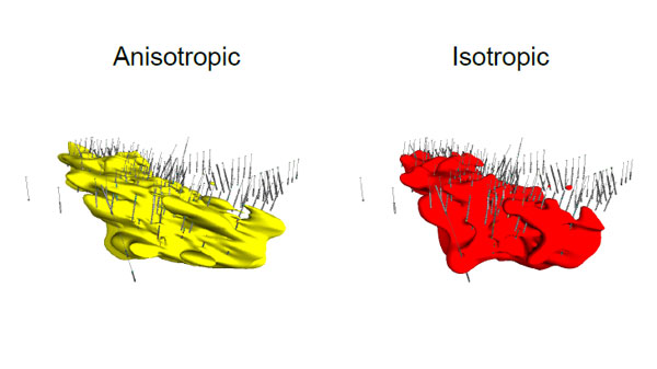 Figure 1. Implicit models of a drillhole dataset using Eureka.
Now to the program under discussion, as mentioned Vulcan 9 has introduced a new module they call Implicit modelling and it comes at no cost for anyone owning the standard geology tools modules. The menu shown below contains the various options available;
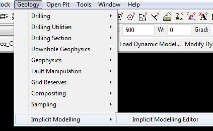
Yep, not many options but what does the Implicit Modelling Editor do?
The editor fires up a standard Vulcan form with a series of options on the left. The first option is the Open Specifications page which allows you to select a parameter file – when selected it will populate all the fields with saved parameters, if you type in a new parameter name the options you enter will be saved in this parameter file.
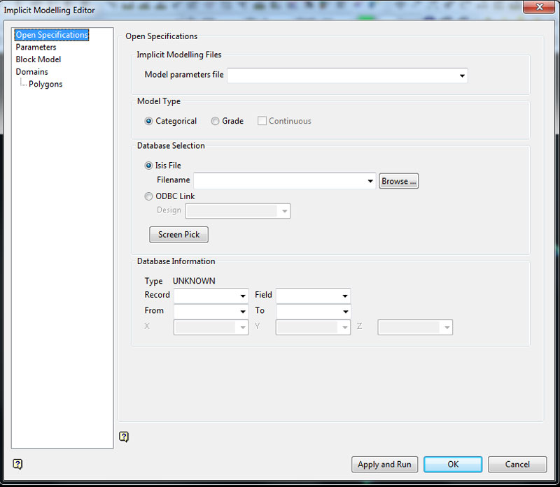
You have the option of selecting a categorical model (such as lithology) or a grade model – which is either categorical (as in indicators) or continuous. You can model from a drillhole database, or from an Isis composite file. If you select from the DH database you are offered the ability to use the data as is or generate a composite file – given the estimate is an ordinary kriged estimate, compositing the data to a regular sample support is recommended. If you do select an already formed composite database you are not required to select a composite length. The database is used to create a distance Map file – a 3D point file that contains the distances away from the “0” point for each category/grade cut-off which is then used to estimate each variable into the blockmodel. Both the Distance_Map file and the blockmodel are written to the project folder. You can either set up a new blockmodel by defining a name and setting up blocksize, origin and extents – or you can select a pre-existing model. Uniquely the distances are negative inside and positive outside – the reverse of that seen in Leapfrog or Micromine.
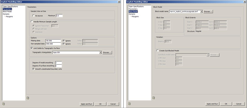
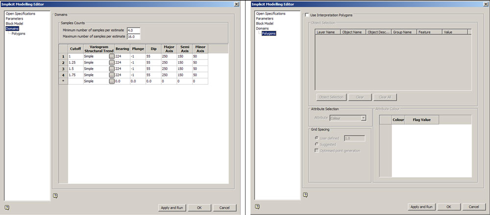
Figure 2. Various options for setting up the estimate.
Like Micromine, Vulcan’s method is technically a local method as it uses a local search as part of the OK estimator and as a result the search parameters need to be set up prior to running the estimate. You can limit the output (as in the categorical shells – not grade shells) to a topographic surface and amend how you want to handle the data, select search parameters and setup a variogram for each category. The variogram can be advanced – as in a standard variogram you have modelled, or you can use a slider that generates a simple variogram that varies between a continuous shape to a smooth shape – not a lot of information on what either option means but it essentially creates a single structure spherical model and adjusts the nugget value. Setting it at very continuous sets the nugget to 5%, very smooth sets the nugget to 95%, ranges are based on the search ellipse you have entered. You can set up min and max number of samples, and adjust the amount of smoothing – both within the model, and within the final output surfaces. You also can use a structural trend and/or a direction of maximum continuity to force and mould the resulting shells.
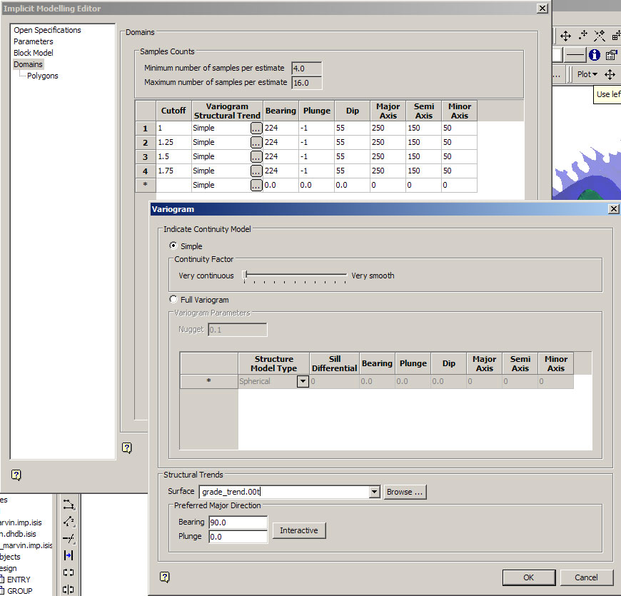 Figure 3. The variogram set-up form, you can also select a triangulation to act as a structural trend to drive the estimate.
The whole process relies on Vulcans block modelling tools to build and then estimate the result into the blockmodel as a distance function, grade shells are then created to generate the output. If you are modelling categorical shells then the shells are meshed together to ensure there are no holes in the model, and they are trimmed to the topography if that has been selected. As the basic block modelling tools are used Vulcan is required to generate a BEF file to control the estimate, and when run you get a standard validation report. Both these files are written to the TMP file on your C: drive and are overwritten every time you create a model. Although the BEF file is a standard file that you can open, edit and adjust it seems you cannot re-run the estimate using the standard estimation process, although you can create distance “grade” shells on the fields in the blockmodel. As an OK estimate it suffers all the foibles of a standard OK estimate, some understanding of the OK estimation process is really required to get a useful output – although it is very easy to generate a basic result.
So what about the results? I have taken the tutorial datasets I used for the Leapfrog-Micromine comparison run them through Vulcan. As for the Micromine comparison; below I present the same comparisons between Leapfrog (using Mining, but Geo outputs the same result) and Vulcan.
Figure 4 shows the results of a basic Isotropic search of the copper variable from Leapfrog’s Marvin dataset. It’s trying is probably as much as you could say for this isotropic result. It must be remembered however that this a very basic no frills unconstrained OK estimate – which for anyone with a bit of experience in this field knows can be very full of pitfalls. With some trial and error and some basic knowledge of the estimation processes and a study of the grade distribution the output looks much better (Figure 5).
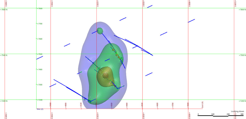
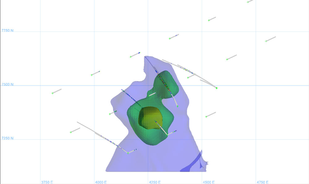
Figure 4. Isotropic search on copper from the Leapfrog Marvin dataset, Leapfrog on the top, Vulcan on the bottom. 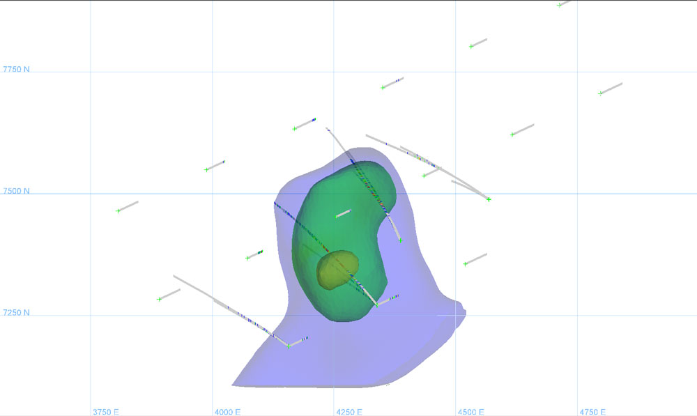 Figure 5. Adjusted estimate using a basic search direction and adjusting the nugget variable in the variogram.
Figure 6 shows the results of using the Lithology modelling. Here like in the Micromine comparison I have modelled the QzP rocktype from the Marvin Dataset. The final output shows similarity between the two. In order to complete the Vulcan surface I have had to play with block size and smoothing but the result is acceptable from a block model domaining point of view. Figure 7 shows the total lithology modelling output when all 3 rocktypes have been modelled. Again given the simplicity of this model the resulting wireframes are quite good and are sufficient for domaining and modelling. More complex models are certainly possible but you are constrained by the fact that you require the blockmodel to create the shells – and thus are required to use an appropriate block sizes. As you are compiling a rocktype estimate and thus have a dataset that is largely continuous (very low nugget) you can get away with blocks that are smaller than you could if doing a grade estimate – blocks of 5-10 times smaller than drillhole spacing (ie 10-20m blocks on 100m spaced drilling) are acceptable, any smaller though and you get artefacts in the wireframes. If you were doing a grade estimate you would be hard pressed to defend blocks any smaller than ¼ drillhole spacing (25m for the 100m spacing) and some would argue you should not go any smaller than ½ (50m).
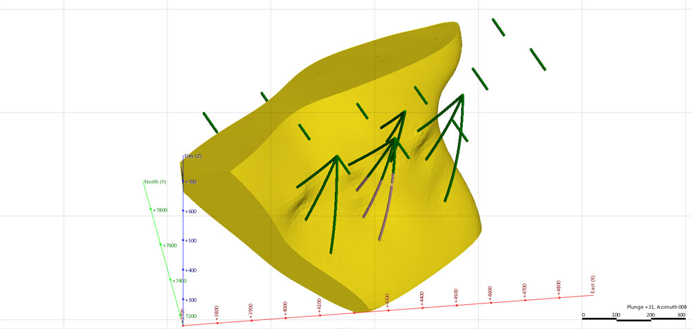
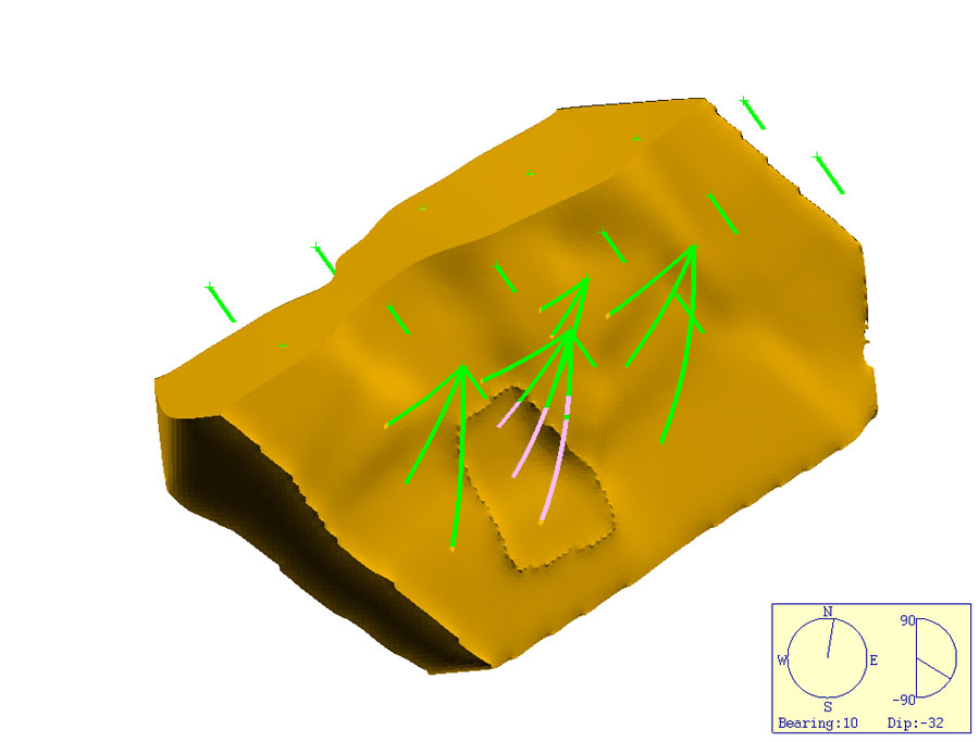
Figure 6. QzP wireframe of the Leapfrog Marvin dataset, Leapfrog on the top, Vulcan on the bottom. 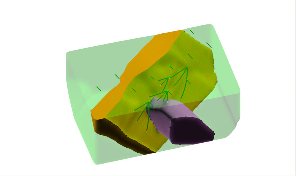 Figure 7. Setting up all the rocktypes in the IM form will build a solid model of the geology, the output for simple geological models such as in the Marvin is quite acceptable.
Figure 8 shows the results of modelling the 5gpt gold grade shell from Micromines NVG dataset using the same anisotropy. From this angle it looks to be OK.
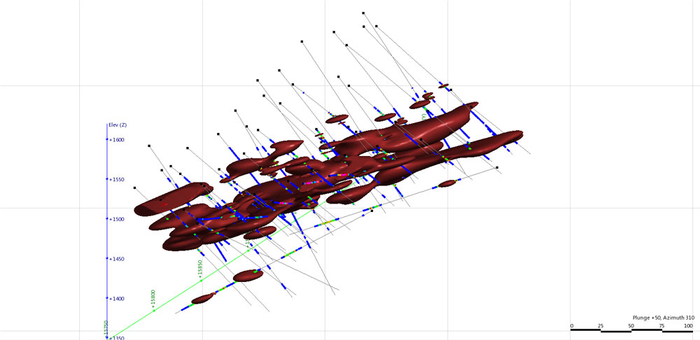
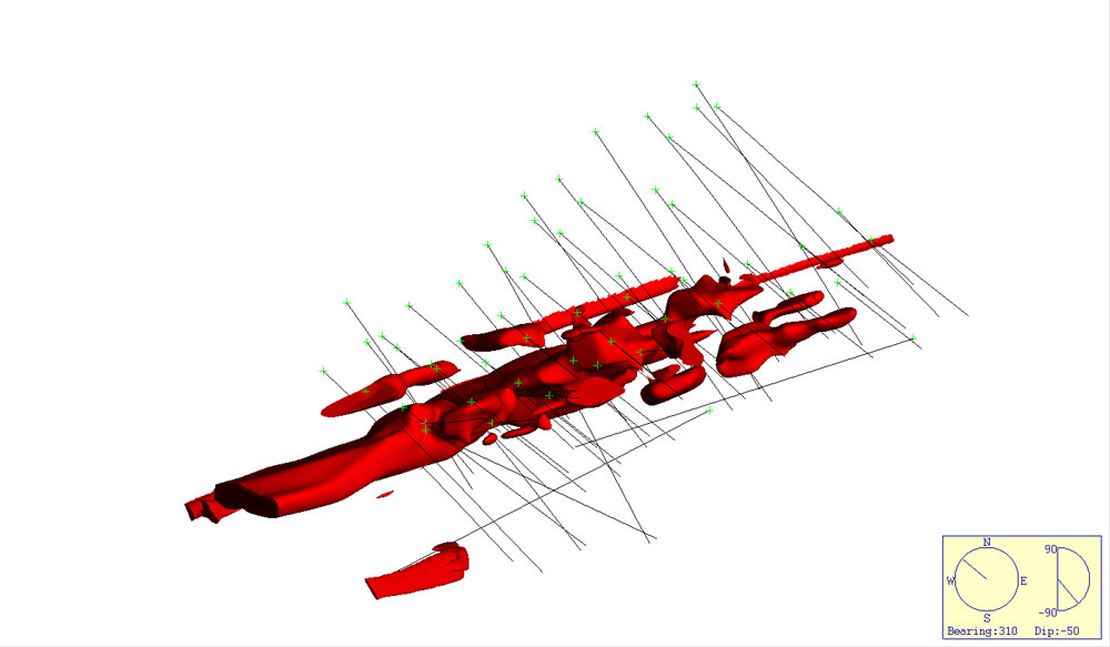
Figure 8. 5gpt shell from the Micromine NVG dataset, Leapfrog on the top, Vulcan on the bottom.
However, when looking normal to this you can see significant estimation errors (Figure 9). This is a by-product of the OK estimation methods used by Vulcan. Playing around with all the various estimation parameters, and the blocksize can reduce these errors but at the loss of definition. A significant amount of the high grade does also get left out of the estimate – again due to this being a standard OK estimate it may mean that blocks in the High Grade areas are more smoothed – and thus lower grade.
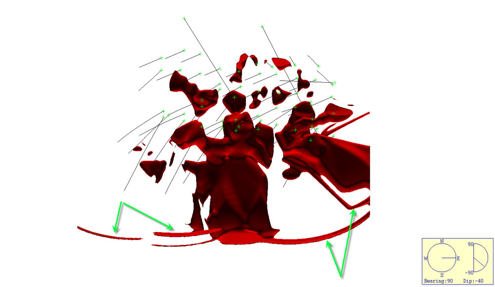 Figure 9. Figure showing the Vulcan estimate normal to the plane of dip, search ellipse artefacts arrowed in green.
Figure 10 shows the results of a largely unguided lithology interpolation of one of the NVG veins, the results from both programs is unacceptable. Whilst I have used an anisotropy for the search both programs have failed to adequately model the vein although the Vulcan option looks more continuous it commonly includes/misses data it should not, at least the Leapfrog program includes all the relevant data.
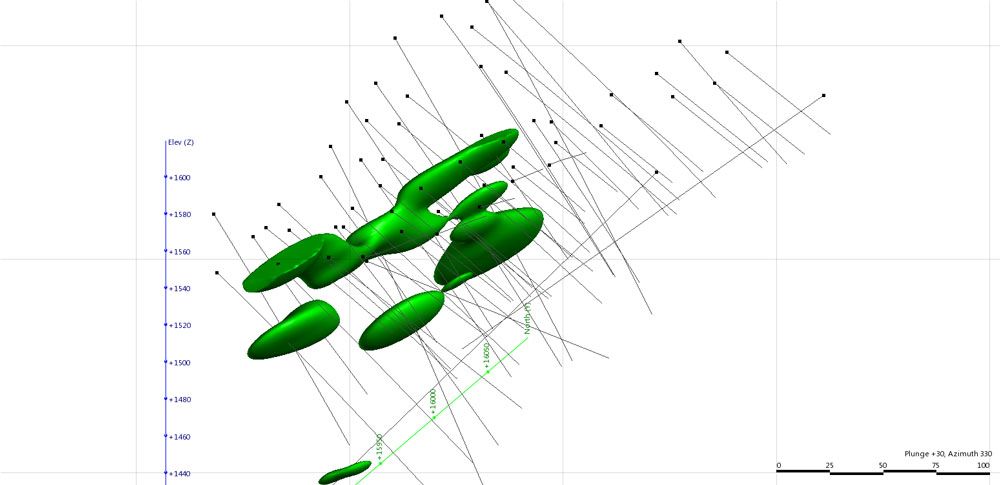
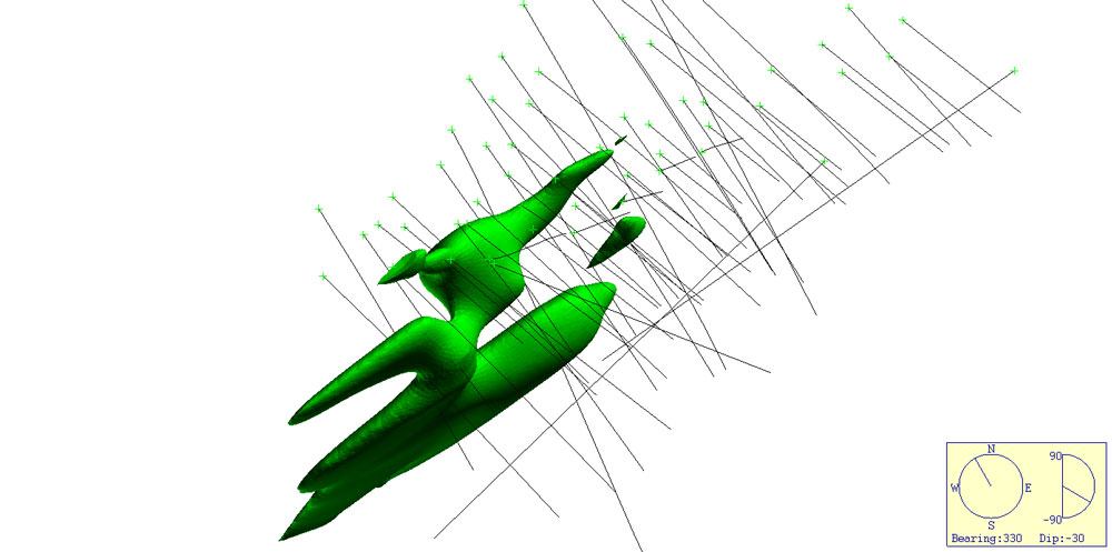
Figure 10. Unguided vein interpolant of a single vein from the Micromine NVG dataset, Leapfrog on the top, Vulcan on the bottom.
Figure 11 however, shows the results using a vein modelling approach. The Leapfrog surface uses an interval selection and the vein modelling methods to drive the interpolation as discussed in the Micromine comparison. With Vulcan I have used every guiding option I can think of when using the interpolator, including using a structural trend surface and polygons – basically an explicit interpretation driving the implicit model. And played with all the various input options, block size, etc. The result is far from acceptable. Although it has to be said that Vulcan does have its own workflows for creating vein models by extracting the footwall and hangingwall points and creating grids which are then meshed together – but these options do not make any use of the “Implicit Modelling” package which is what I am reviewing here.
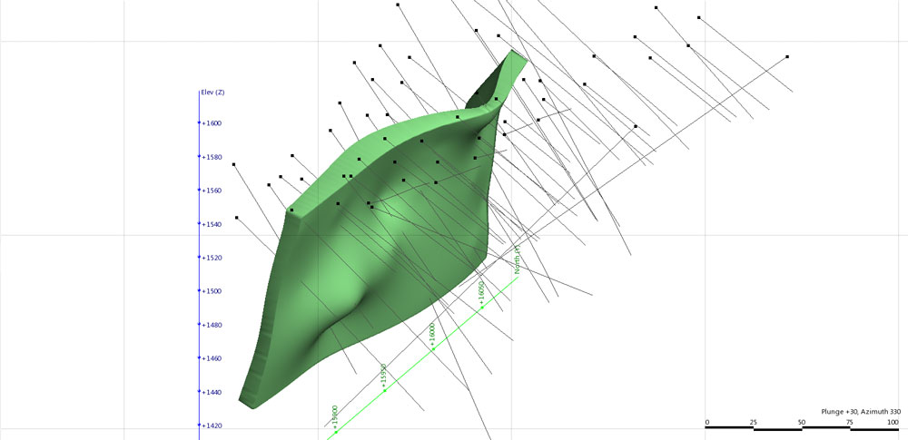
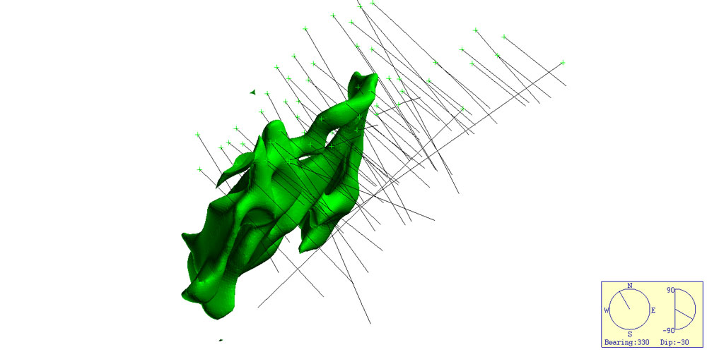
Figure 11. The same vein from the Micromine NVG dataset, Leapfrog using vein modelling on the top, Vulcan using structural trend modelling and polygons on the bottom.
In the final analysis, whilst the output for Vulcan is generally acceptable from a basic 3D geological model generation point of view as demonstrated with the Marvin dataset it struggles when handling the more complex geological architecture indicated in the NVG dataset. Leapfrogs ability to handle complex datasets; its rapid shell generation, its true RBF method and data analysis capability is a significant factor in its favour. Vulcan however requires quite a bit more set up and planning getting to the same point, additionally some basic understanding of kriging and its pitfalls is a requirement in getting a final end product.
Geological models in Leapfrog use domains (in the case of LF Mining) or Geology Models (in the case of LF Geo) to create a solid 3D geology model with inbuilt overprinting and stratigraphic relationships. In Vulcan you use the geology in the logging to manually define each of the rocktypes and these are then modelled and meshed together en-mass. The process does give an acceptable result from a block model point of view (again if the domains are simple) but has significant problems modelling more complex data.
In its current form Vulcan’s Implicit Modeller is much more advanced and capable grid based traditional system than GeoVia’s Dynamic Shells. It is a tool that would be of benefit to the resource geologist looking to develop a series of resource domains on large bulk style deposits (copper porphyries for instance) where geometries are simple and overprinting relationships are not significant. The ability to generate simple grade shells, and basic domains allows you to flag up a block model with the domains and then flag and extract the composites for statistical analysis. As a component in the resource modelling workflow it might be useful. Also from a basic broad scale assessment of a deposit it might also be helpful. It does however struggle with more complex deposits where the RBF approach really comes into its own. Leapfrog and Micromine do a much better job of handling these sorts of deposits – gold for example, and are much more versatile when it comes to 3D modelling of larger province or camp scale models. If Maptek can implement the RBF method that has been added to the Eureka software into Vulcan I think there will be a measurable improvement in the IM module.
All in all I think the IM module is a useful addition to the Vulcan Package, and as it comes standard with the basic geology modules may get a lot more use (and thus feedback for future development) than where you are required to pay for the privilege. However, outside the resource geologist playing around with domains and obtaining a first pass looksee I think it has little to offer but the ground work and potential is certainly there for Vulcan to become a significant player in the field.
Is this implementation true “Implicit Modelling”, I think not as I feel you require some form of RBF or similar process (- the “rubber band effect”) to truly be called Implicit – although there are others who argue that if it creates a model without using explicitly digitised strings then it is by definition implicit. These arguments are probably circular and will have a ways to go before they are truly settled and I think for now I will stick with my own probably biased opinion.